Submodels vs Elementary Submodels

01 Oct 2020

I’m giving a GSS talk next week in the hopes of introducing myself to my new department. More importantly, I am giving this talk to try and showcase the utility of model theory in combinatorics and algebra. While writing this talk, I’ve been thinking about the best way to discuss elementary submodels as opposed to regular old submodels. When it was taught to me, a focus was placed on “quantifying over extra stuff”, which is true, but I was never shown a simple example. While I was thinking about how to teach it, I realized we can already find elementary and nonelementary submodels in graph theory, and that these might serve as good examples for people new to the area.

So, to begin, we have to talk about Models. I’m planning to write a longer form post on model theory at some point, but here are the basics.

We typically have functions, relations, and constants associated to any given “structure” in mathematics. For groups, we obviously have the constant $e$ (representing the identity), a binary function $\cdot$ (for the group operation), and a unary function ${}^{-1}$ (for inversion). We can define other operations too, such as the commutator $[x,y]=x^{-1}{y}^{-1}xy$, but these can all be defined in terms of the operations given. For the natural numbers $\mathbb{N}$ we often restrict our attention to the constants $0$ and $1$, as well as binary functions $+$ and $\times$, and a relation $\le \subseteq {\mathbb{N}}^2$. An example that we will refer to for the rest of this post will be graphs. A graph has a single binary relation $E$ – the edge relation.

When studying any fixed branch of math, the discourse is usually confied to formulas involving only some collection of symbols. Often we prove things by manipulating these symbols according to known rules, which are set out in axioms for how these symbols should behave. Model Theory studies what we can prove using only this information, and by formulating certain problems model theoretically, we can bring a lot of powerful machinery to bear.

---

To start, we have to fix the symbols of interest. A Signature is a tuple $\sigma =(C,R_{\bullet },F_{\bullet })$, where $C$ is a set of Constant Symbols, $R_n$ is a set of (n-ary) Relation Symbols, and $F_n$ is a set of (n-ary) Function Symbols.

Then we can define the Language $\mathcal{L}(\sigma )$ as (informally) the set of mathematical formulas using

• symbols from $\sigma$
• variables $x_1,x_2,x_3,\dots$
• =
• $\wedge$, $\vee$, $\mathrm{\neg }$, $\to$, $\leftrightarrow$
• $\mathrm{\forall }$, $\mathrm{\exists }$

From your mathematical experience, you doubtless know intuitively how these symbols are allowed to fit together. However, for those wanting to see the precise definition, I’ve included one at this footnote ¹.

Now that we know what formulas we are allowed to discuss (in a fixed language $\mathcal{L}(\sigma )$), it is time to discuss models for this language. These models are sets equipped with functions and relations for each symbol in $\sigma$, and will give us a way to assign a truth value to formulas.

Formally, a $\sigma$-model $\mathfrak{M}=(M,C^{\mathfrak{M}},R_{\bullet }^{\mathfrak{M}},F_{\bullet }^{\mathfrak{M}})$ is a set $M$ plus an element $c^{\mathfrak{M}}\in M$ for each $c\in C$, a function $f^{\mathfrak{M}}:M^n\to M$ for each (n-ary) $f\in F_n$, and a relation $r^{\mathfrak{M}}\subseteq M^n$ for each (n-ary) $r\in R_n$. In practice, the superscript $\mathfrak{M}$ is often omitted when the model is clear from context.

Now that we know how to interpret the symbols of $\sigma$, it is intuitively clear how to bootstrap our way to an interpretation of the formulas of $\mathcal{L}(\sigma )$. One uses the traditional meantings of the extra symbols, and asks whether the resulting formula is true in $M$. This is perhaps best given as a “definition by example” (which I’ll provide in the next paragraph), but I have again left a formal definition as a footnote ².

Let’s look at the signature $\sigma$ with one constant $0$, a binary function $+$, and a binary relation $\le$. Then we can take the set $\mathbb{N}$ with the obvious interpretation as a $\sigma$-model. Let’s take $\phi =\mathrm{\forall }m.\mathrm{\exists }n.n\ge m$ as a case study. $\mathbb{N}$ obviously thinks this formula is true, because for all $m\in \mathbb{N}$ there does exist a $n\in \mathbb{N}$ so that $n{\ge }^{\mathbb{N}}m$. In this case, we write $\mathbb{N}\models \phi$, which we read as “$\mathbb{N}$ models $\phi$” or, “$\mathbb{N}$ satisfies $\phi$”, or “$\mathbb{N}$ thinks that $\phi$ is true”, etc. If instead we look at $\psi =\mathrm{\exists }n.\mathrm{\forall }x.x+n=0$, we see that $\psi$ is false in $\mathbb{N}$. This is because, no matter which $n\in \mathbb{N}$ you pick, there is always an $x\in \mathbb{N}$ so that $n{+}^{\mathbb{N}}x\ne 0^{\mathbb{N}}$. In this instance, we say $\mathbb{N}⊭\psi$.

Notice, however, that there is no restriction (yet) on our interpretation. We could look at a nonstandard interpretation, say $\tilde{\mathbb{N}}$, where $0^{\tilde{\mathbb{N}}}=3$, $x{+}^{\tilde{\mathbb{N}}}y=3$ for every $x$ and $y$, and ${\le }^{\tilde{\mathbb{N}}}=\{(4,5)\}$. Then we see $\tilde{\mathbb{N}}⊭\phi$, and $\tilde{\mathbb{N}}\models \psi$ (why?). We could even work with a totally different set, and look at $M=\{a,b,c\}$ with $0^{\mathfrak{M}}=a$, ${\le }^{\mathfrak{M}}=\{(a,b),(c,b)\}$, and $x{+}^{\mathfrak{M}}y=b$. Obviously this example was arbitrary, so you can imagine the diversity of possible models.

In practice, though, we almost never work with bare models. We always ask that our models satisfy some axioms $A\subseteq \mathcal{L}(\sigma )$. These axioms greatly restrict which models we view as worthy of study, but we still view them abstractly. A very common technique in model theory is to add symbols and axioms to a theory of interest. Then we use these extra symbols and axioms to force our model to behave in a certain way (after arguing that such a model must exist). Then we “forget” about the extra symbols, and see that this new model is still a model of our original theory, but it has new properties that are desirable.

---

Today, though, we’re not talking about these techniques. We are instead focusing on two notions of “submodel”, and talking about their differences. We will focus on graphs, since they are simple combinatorial objects that one can easily understand and play with. For us, a graph will be a model for the signature $G$ with exactly one binary relation $E$. Moreover, we will restrict attention to those models satisfying the symmetry axiom $\mathrm{\forall }x.\mathrm{\forall }y.xEy⟹yEx$. If you would rather your graphs be loopless, we could also add the irreflexivity axiom $\mathrm{\forall }x.\mathrm{\neg }xEx$, but this will not be relevant for our discussion.

A submodel $\mathfrak{X}$ of a $\sigma$-model $\mathfrak{M}$ is almost certainly what you’re expecting. It is a subset $X\subseteq M$ which contains all the constants in $C$ and is closed under all the functions in $F_{\bullet }$. Then we can define $c^{\mathfrak{X}}=c^{\mathfrak{M}}$, $f^{\mathfrak{X}}=f^{\mathfrak{M}}\upharpoonright X^n$, and $r^{\mathfrak{X}}=r^{\mathfrak{M}}\cap X^n$. The only important (and sometimes counterintuitive) part of this definition is the notion of relation. This is best shown by a graph theoretic example.

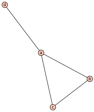
Consider the following graph $\mathrm{\Gamma }$, which we view as a $G$-model:

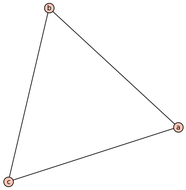
Then submodels are the induced or full subgraphs. Notably this is a submodel:

While this (the tripod $T$) isn’t:

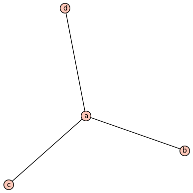
This fails to be a submodel beacsue its edge relation $E^T$ is not equal to $E^{\mathrm{\Gamma }}\cap \{a,b,c,d{\}}^2$. Model theory has a way to talk about these kinds of “almost submodels”, though. The inclusion $i:T\hookrightarrow \mathrm{\Gamma }$ is a homomorphism of models, and homomorhpisms have to preserve “positive formulas” (roughly, the formulas with no $\mathrm{\neg }$ and no quantifiers). The converse fails, however, and we can see $T\models \mathrm{\neg }bEc$ while $\mathrm{\Gamma }⊭\mathrm{\neg }i(b)Ei(c)$.

As an algebraic example, consider the natural homomorphism $p$ from a group to its abelianization. If some element $g$ is of order $n$, then its image $p(g)$ will still be of order $n$. We can think of this is reflecting that whenever $G\models g^n=1$, we also have $G^{\text{ab}}\models p(g{)}^n=1$. Any relations among the elements of $g$ are preserved by the homomorphism. These are the “positive formulas”. Statements about what things aren’t related, though, might fail to be preserved. For instance, if $g$ and $h$ don’t commute in $G$, we will have $G\models gh\ne hg$, while $G^{\text{ab}}\models p(g)p(h)=p(h)p(g)$. Existing relations must be preserved, but homomorphisms are allowed to add new relations.

Submodels, though (and more generally embeddings) preserve positive and negative formulas. Phrased differently, submodels both preserve and reflect positive formulas. Phrased differently yet again, if $\mathfrak{X}$ is a submodel of $\mathfrak{M}$ then for every quantifier free formula $\phi$ and every $a_1,\dots ,a_n\in X$ we have

$$\mathfrak{X}\models \phi (a_1,\dots ,a_n)⟺\mathfrak{M}\models \phi (a_1,\dots ,a_n)$$

But what, I hear you asking, about quantifiers? Notice it is not true that submodels have to prserve the truth of formulas with quantifiers. Intuitively, think about a formula $\mathrm{\exists }x.\phi$. It is entirely possible that such an $x$ exists in $\mathfrak{M}$ but that element was excluded from the submodel. Similarly, it might be the case that $\mathfrak{X}$ thinks that $\mathrm{\forall }x.\phi$, simply because we excluded all of the counterexamples which might exist in $\mathfrak{M}$!

As a concrete example, consider the center $Z(G)$ of a group $G$. This is a submodel, but $Z\models \mathrm{\forall }x.\mathrm{\forall }y.xy=yx$, while $G$ (typically) does not. Perhaps even more agressively, we have $G\models \mathrm{\exists }x.x\ne e$, while the trivial subgroup $1\le G$ doesn’t!

We can see similar behavior in graphs. For instance, the following graph has $\mathrm{\Gamma }\models \mathrm{\exists }x.\mathrm{\forall }y.x\ne y\to xEy$.

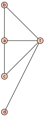
However, the submodel which excludes $t$ does not satisfy that formula.

---

This brings us to a very special kind of submodel. A submodel $\mathfrak{X}$ of $\mathfrak{M}$ is caled elementary if and only if, given any elements $a_1,\dots ,a_n\in X$ and any formula $\phi$ at all,

$$\mathfrak{X}\models \phi (a_1,\dots ,a_n)⟺\mathfrak{M}\models \phi (a_1,\dots ,a_n).$$

To show that a submodel is elementary, we have the Tarski-Vaught Test, which says that $\mathfrak{X}$ is an elementary substructure of $\mathfrak{M}$ if and only if for every $a_1,\dots ,a_n\in X$ and for every $\phi$: whenever some $m\in M$ satisfies $\phi (m,a_1,\dots ,a_n)$, there is already a $m^{\prime }\in X$ which also satisfies $\phi (m^{\prime },a_1,\dots ,a_n)$. This says that anytime we can find an element in $M$ that makes a formula true, we can actually do it without leaving $X$.

One easy example of an elementary submodel is $K_{\mathbb{N}}$, the complete graph with one vertex for each natural number, as a submodel of $K_{\mathbb{Z}}$, the complete graph with one vertex for each integer. These are both isomorphic to $K_{{\mathrm{\aleph }}_0}$, and thus they are isomorphic to each other. It is clear, then, that they have the same first order theory.

Since an elementary submodel $\mathfrak{X}$ must look almost exactly like the full structure $\mathfrak{M}$, you might think that this is the only possibility. You might think there must be an isomorphismm $\mathfrak{X}\cong \mathfrak{M}$. Thankfully (and surprisingly!) this is false! This is the source of lots of interesting mathematics.

To get an example of this phenomenon, we can generalize the above example slightly. Look at $K_{\mathbb{N}}$ again, but now viewed as a subgraph of $K_{\mathbb{R}}$ (the complete graph with one vertex for each real number). Clearly these aren’t isomorphic, since they have different cardinalities. On the other hand, it is intuitively clear that they look extremely similar, especially since any fixed formula can only refer to finitely many vertices (or, with a quantifier, all vertices at once).

As a second, less trivial example, consider the following graph $\mathrm{\Gamma }$ of integers, where $x$ and $y$ are adjacent whenever their difference is $\pm 1$. Obviously the graphic shows only a finite part of the infinite graph.

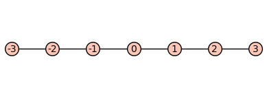
We can also consider the disjoint union $\mathrm{\Gamma }+\mathrm{\Gamma }$ of two such graphs. Again, we only show a finite part of this graph.

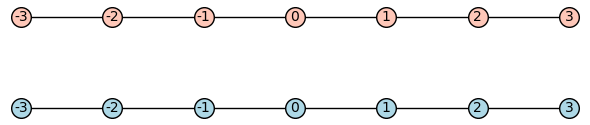
It turns out $\mathrm{\Gamma }$ and $\mathrm{\Gamma }+\mathrm{\Gamma }$ are elementary equivalent! (can you show this with the Tarski-Vaught Test?) Then no first order logic formula can detect disconnectedness. If $G\models \phi$ were true if and only if $G$ is connected, then $\mathrm{\Gamma }\models \phi$ while $\mathrm{\Gamma }+\mathrm{\Gamma }⊭\phi$. But since $\mathrm{\Gamma }$ and $\mathrm{\Gamma }+\mathrm{\Gamma }$ have the same first order theory, no such $\phi$ can exist! Intuitively, this is because any first order formula can only say “there is no path of length n”, which doesn’t exclude the possibility of some longer path. If you choose to prove the first graph is an elementary submodel of the second using vaught’s test, you’ll make this intuition formal. Any existential statement which is witnessed by something in the other copy of $\mathbb{Z}$ can actually be witnessed by something in the same copy of $\mathbb{Z}$ that’s far enough away.

There are lots of reasons elementary submodels are useful (for a famous example, see nonstandard analysis ), but it’s important to keep straight the difference between homomorphic images, submodels, and elementary submodels. I know I was tripped up by this for a long time, and a younger me would have been helped by these toy examples from graph theory.

---