Measure Theory and Differentiation (Part 1)

21 Feb 2021 - Tags: measure-theory-and-differentiation , analysis-qual-prep

So I had an analysis exam yesterday last week a while ago (this post took a bit of time to finish writing). It roughly covered the material in chapter 3 of Folland’s “Real Analysis: Modern Techniques and Their Applications”. I’m decently comfortable with the material, but a lot of it has always felt kind of unmotivated. For example, why is the Lebesgue Differentiation Theorem called that? It doesn’t look like a derivative… At least not at first glance.

A big part of my studying process is fitting together the various theorems into a coherent narrative. It doesn’t have to be linear (in fact, it typically isn’t!), but it should feel like the theorems share some purpose, and fit together neatly. I also struggle to care about theorems before I know what they do. This is part of why I care so much about examples – it’s nice to know what problems a given theorem solves.

After a fair amount of reading and thinking¹, I think I’ve finally fit the puzzle pieces together in a way that works for me. Since I wrote it all down for myself as part of my studying, I figured I would post it here as well in case other people find it useful. Keep in mind this is probably obvious to anyone with an analytic mind, but it certainly wasn’t obvious to me!

Let’s get started!

---

To start, we need to remember how to relate functions and measures. Everything we say here will be in $\mathbb{R}$, and $m$ will be the ($1$-dimensional) Lebesgue Measure.

This is more or less the content of the Carathéodory Extension Theorem. It’s worth taking a second to think where we use the assumptions on $F$. The fact that $F$ is increasing means our measure is positive. Continuity from the right is a bit more subtle, though. Since $F_{\mu }$ is always right continuous, we need to assume our starting function is right continuous in order to guarantee $F_{{\mu }_F}=F$.

This is not a big deal, though. A monotone function is automatically continuous except at a countable set (see here for a proof) and at its countably many discontinuities, we can force right-continuity by defining

$$\tilde{F}(x_0)\triangleq \underset{x\to x_0^{+}}{lim}F(x)$$

which agrees with $F$ wherever $F$ is continuous. If we put our probabilist hat on, we say that $F_{\mu }$ is the Cumulative Distribution Function of $\mu$. Here $F_{\mu }(x)$ represents the total (cumulative) mass we’ve seen so far.

It turns out that Lebesgue-Stieltjes measures are extremely concrete, and a lot of this post is going to talk about computing with them². After all, it’s entirely unclear which (if any!) techniques from a calculus class carry over when we try to actually integrate against some ${\mu }_F$. Before we can talk about computation, though, we have to recall another (a priori unrelated) way to relate functions to measures:

The locally $L^1$ conditions says that ${\int }_{E}fdm$ is finite whenever $E$ is bounded. It’s not hard to show that this is equivalent to the regularity of $m_f$, which we’ll need shortly.

Something is missing from the above theorem, though. We know sending $F⇝{\mu }_F$ is faithful, in the sense that $F=F_{{\mu }_F}$ and ${\mu }_{F_{\mu }}=\mu$. We’ve now introduced the measure $m_f$, but we didn’t say how to recover $f$ from $m_f$… Is it even possible? The answer is yes, as a corollary of a much more powerful result:

In the case $\mu =m_f$, then this shows us how to recover $f$ (uniquely) from $m_f$, and life is good:

$$\frac{d{m}_f}{dm}=f$$

The converse needs a ~bonus condition~. In order to say $\mu =m_{\frac{d\mu }{dm}}$, we need to know that $\mu$ is absolutely continuous with respect to $m$, written $\mu \ll m$.

In the case of Lebesgue-Stieltjes measures, Lebesgue-Radon-Nikodym buys us something almost magical. For almost every $x$, we see:

$$\begin{array}{rl}\frac{d{\mu }_F}{dm}(x)& =\underset{r\to 0}{lim}\frac{{\mu }_F(B_r(x))}{m(B_r(x))}\\ & =\underset{r\to 0}{lim}\frac{F(x+r)-F(x-r)}{x+r-(x-r)}\\ & =\underset{r\to 0}{lim}\frac{F(x+r)-F(x-r)}{2r}\\ & =F^{\prime }(x)\end{array}$$

Now we see why we might call this $f$ the Radon-Nikodym derivative. In the special case of Lebesgue-Stieltjes measures, it literally is the derivative. It’s immediate from the definitions that $F=F_{m_f}$ acts like an antiderivative of $f$, since $F_{m_f}(x)={\int }_0^{x}fdm$. Now we see $f=\frac{d{\mu }_F}{dm}$ works as a derivative of $F$ as well!

In fact, we can push this even further! Let’s take a look at the Lebesgue Differentiation Theorem

Why is this called the differentiation theorem? Let’s look at $F_{m_f}$, which you should remember is a kind of antiderivative for $f$.

For $x>0$ (for simplicity), we have $F_{m_f}(x)=m_f((0,x])={\int }_{(0,x]}fdm$. If we rewrite the theorem in terms of $F_{m_f}$, what do we see?

$$\begin{array}{rl}f(x)& =\underset{r\to 0}{lim}\frac{1}{m{B}_r(x)}{\int }_{B_r(x)}fdm\\ & =\underset{r\to 0}{lim}\frac{1}{(x+r)-(x-r)}{\int }_{x-r}^{x+r}fdm\\ & =\underset{r\to 0}{lim}\frac{1}{2r}({\int }_0^{x+r}fdm-{\int }_0^{x-r}fdm)\\ & =\underset{r\to 0}{lim}\frac{F_{m_f}(x+r)-F_{m_f}(x-r)}{2r}\\ & =F_{m_f}^{\prime }(x)\end{array}$$

So this is giving us part of the fundamental theorem of calculus⁴! This theorem (in the case of Lebesgue-Stieltjes measures) says exactly that (for almost every $x$)

$${(x\mapsto {\int }_0^{x}fdm)}^{\prime }=f(x)$$

Let’s take a moment to summarize the relationships we’ve seen. Then we’ll use these relationships to actually compute with Lebesgue-Stieltjes integrals.

---

Why should we care about these theorems? Well, Lebesgue-Stieltjes integrals arise fairly regularly in the wild, and these theorems let us actually compute them! It’s easy to integrate against $m_f$, since monotone convergence gives us $\int gd{m}_f=\int gfdm$.

Then this buys us the (very memorable) formula:

$$\int gd{\mu }_F=\int g\frac{d{\mu }_F}{dm}dm=\int g{F}^{\prime }dm$$

and now we’re integrating against lebesgue measure, and all our years of calculus experience is applicable!

Of course, I’ve left out an important detail: Whatever happened to that measure $\lambda$? The above formula is true exactly when $F$ is continuous everywhere. At points where it is discontinuous we need to change it slightly by using $\lambda$. These are called singular measures, and they can be pretty pathological. A good first intuition, though, is to think of them like dirac measures, and that’s the case that we’ll focus on in this post⁵.

Let’s write $H=\{\begin{array}{ll}0& x<0\\ 1& 0\le x\end{array}$. This us usually called the heaviside function.

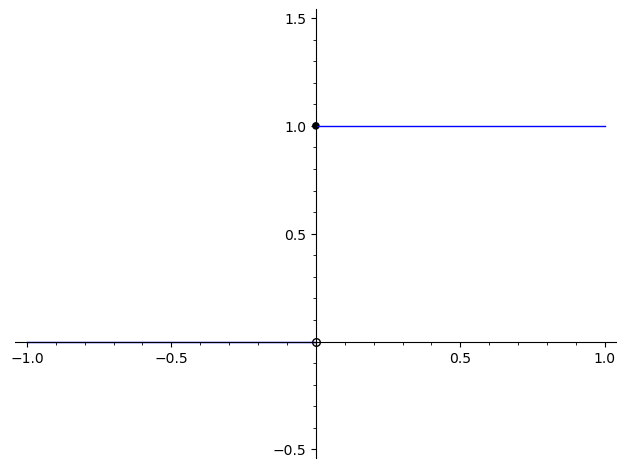
Recall our interpretation of this function: $H(x)$ is supposed to represent the mass of $(-\mathrm{\infty },x]$. So as we scan from left to right, we see the mass is constantly $0$ until we hit the point $0$. Then suddenly we jump up to mass $1$. But once we get there, our mass stays constant again.

So $H$ thinks that $0$ has mass $1$ all by itself, and thinks that there’s no other mass at all!

Indeed, we see that

$${\mu }_H((a,b])=H(b)-H(a)=\{\begin{array}{ll}1& 0\in (a,b]\\ 0& 0\notin (a,b]\end{array}$$

So ${\mu }_H$ is just the dirac measure at $0$ (or ${\delta }_0$ to its friends)! Notice this lets us say the “derivative” of $H$ is ${\delta }_0$, by analogy with the Lebesgue-Stieltjes case. Or conversely, that $H$ is the “antiderivative” of ${\delta }_0$. This shows us that recasting calculus in this language actually buys us something new, since there’s no way to make sense of ${\delta }_0$ as a traditional function.

It’s finally computation time! Since we know $\int gd{\delta }_0=g(0)$, and (discrete) singular measures look like (possibly infinite) linear combinations of dirac measures, this lets us compute all increasing right-continuous Lebesgue-Stieltjes measures that are likely to arise in practice. Let’s see some examples! If you want to see more, you really should look into Carter and van Brunt’s “The Lebesgue-Stieltjes Integral: A Practical Introduction”. I mentioned it in a footnote earlier, but it really deserves a spotlight. It’s full of concrete examples, and is extremely readable!

---

Let’s start with a continuous example. Say $F=\{\begin{array}{ll}0& x\le 0\\ x^2& x\ge 0\end{array}$.

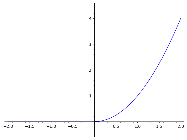
So ${\mu }_F$ should think that everything is massless until we hit $0$. From then on, we start gaining mass faster and faster as we move to the right. If you like, larger points are “more dense” than smaller ones, and thus contribute more mass in the same amount of space.

Say we want to compute

$${\int }_{-\pi }^{\pi }\sin (x)d{\mu }_F={\int }_{-\pi }^{\pi }\sin (x)\cdot F^{\prime }dm$$

We can compute $F^{\prime }=\{\begin{array}{ll}0& x\le 0\\ 2x& x\ge 0\end{array}$, so we split up our integral as

$${\int }_{-\pi }^0\sin (x)\cdot 0dm+{\int }_0^{\pi }\sin (x)\cdot 2xdm$$

But both of these are integrals against lebesgue measure $m$! So these are just “classical” integrals, and we can use all our favorite tools. So the first integral is $0$, and the second integral is $2\pi$ (integrating by parts). This gives

$${\int }_{-\pi }^{\pi }\sin (x)d{\mu }_F=2\pi$$

That wasn’t so bad, right?

---

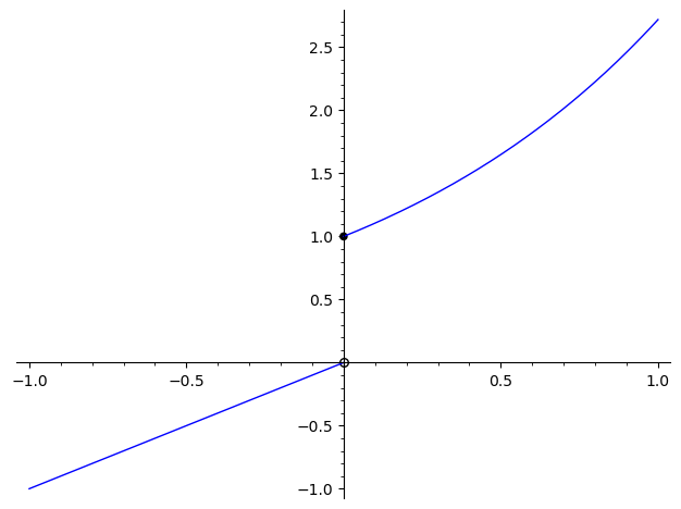
Let’s see another, slightly trickier one. Let’s look at $F=\{\begin{array}{ll}x& x<0\\ e^x& x\ge 0\end{array}$

You should think through the intuition for what ${\mu }_F$ looks like. You can then test your intuition against a computation:

$${\mu }_F=\lambda +m_f$$

In the previous example, $\lambda$ was the $0$ measure since our function was differentiable everywhere. Now, though, we aren’t as lucky. Our function $F$ is not differentiable at $0$, so we will have to work with some nontrivial $\lambda$.

Let’s start with the places $F$ is differentiable. This gives us the density function $f=F^{\prime }=\{\begin{array}{ll}1& x<0\\ e^x& x>0\end{array}$.

We can also see the point $0$ has mass $1$. In this case we can more or less read this off the graph (since we have a discontinuity where we jump up by $1$), but in more complex examples we would compute this by using ${\mu }_F(0)=\underset{r\to 0^{+}}{lim}F(r)-F(-r)$. You can see that this does give us $1$ in this case, as expected. So we see (for $f$ as before)

$${\mu }_F={\delta }_0+m_f$$

So to compute

$${\int }_{-1}^{1}4-x^{2}d{\mu }_F={\int }_{-1}^{1}4-x^{2}d({\delta }_0+m_f)={\int }_{-1}^{1}4-x^{2}d{\delta }_0+{\int }_{-1}^1(4-x^2)fdm$$

we can handle the ${\delta }_0$ part and the $fdm$ part separately!

We know how to handle dirac measures:

$${\int }_{-1}^{1}4-x^{2}d{\delta }_0={(4-x^2)|}_{x=0}=4$$

And we also know how to handle “classical” integrals:

$${\int }_{-1}^1(4-x^2)fdm={\int }_{-1}^0(4-x^2)dm+{\int }_0^1(4-x^2)e^{x}dm=\frac{11}{3}+(3e-2)$$

So all together, we get ${\int }_{-1}^{1}4-x^{2}d{\mu }_F=4+\frac{11}{3}+(3e-2)$.

---

Ok, I hear you saying. There’s a really tight connection between increasing (right-)continuous functions $F$ on $\mathbb{R}$ and positive integrable functions $f$. This connection is at its tightest wherever $F$ is actually continuous, as then the measures ${\mu }_F$ and $m_f$ have a derivative relationship, which is reflected in the same derivative relationship of functions $F^{\prime }=f$. Not only does this give us a way to generalize the notion of derivative to functions that might not normally have one (as in the case of the heaviside function and the dirac delta), it gives us a concrete way of evaluating Lebesgue-Stieltjes integrals.

But doesn’t this feel restrictive? There are lots of functions $F$ which aren’t (right-)continuous or increasing that we might be interested in differentiating. There are also lots of nonpositive functions $f$ which we might be interested in integrating. Since we got a kind of “fundamental theorem of calculus” from these measure theoretic techniques, if we can show how to apply these techniques to a broader class of functions, we might be able to get a more general fundamental theorem of calculus.

Of course, to talk about more general functions $F$, we’ll need to allow our measures to assign negative mass to certain sets. That’s ok, though, and we can even go so far as to allow complex valued measures! In fact, from what I can tell, this really is the raison d’être for signed and complex measures. I was always a bit confused why we might care about these objects, but it’s beginning to make more sense.

This post is getting pretty long, though, so we’ll talk about the signed case in a (much shorter, hopefully) part 2!

---