Cohomology Intuitively

01 Mar 2021 - Tags: cohomology-intuitively , sage , featured

So I was on mse the other day…

Anyways, somebody asked a question about finding generators in cohomology groups. I think understanding how to compute the generators is important, but it’s equally important to understand what that computation is doing. Regrettably, while there’s some very nice visual intuition¹ for homology classes and what they represent, cohomology groups tend to feel a bit more abstract.

This post is going to be an extension of the answer I gave on the linked question. Cohomology is a big subject, and there were a lot of things that I wanted to include in that answer that I didn’t have space for. A blog post is a much more reasonable setting for something a bit more rambling anyways. That said, everything contained in that answer will also be discussed here, so it’s far from prerequisite reading.

In particular, we’re going to go over Simplicial Cohomology², but we’ll steal language from De Rham Cohomology, and our first example will be a kind of informal cohomology just to get the idea across.

There’s a really nice example that Florian Frick gave when I took his algebraic topology class, and it was such good pedagogy I have to evangelize it. The idea is to study simplicial cohomology for graphs – it turns out to say something which is very down to earth, and we can then view cohomology of more complicated simplicial complexes as a generalization of this.

Graphs are one of very few things that we can really understand, and so using them as a case study for more complex theorems tends to be a good idea. As such, we’ll study what cohomology on graphs is all about, and there will even be some sage code at the bottom so you can check some small cases yourself!

With that out of the way, let’s get started ^_^

First things first. Let’s give a high level description of what cohomology does for us.

Say you have a geometric object, and you want to define a function on it. This is a very general framework, and “geometric” can mean a lot of different things. Maybe you want to define a continuous function on some topological space. Or perhaps you’re interested in smooth functions on a manifold. The same idea works for defining functions on schemes as well, and the rabbit hole seems to go endlessly deep!

For concreteness, let’s say we want to define a square root function on the complex plane. So our “geometric object” will be $C$ and our goal will be to define a continuous $\sqrt{\cdot}$ on it.

It’s often the case that you know what you want your function to do somewhere (that’s why we want to define it at all!), and then you would like to extend that function to a function defined everywhere.

For us, then, we know we want $\sqrt{1} = 1$ .

This is an arbitrary choice, but it certainly seems like a natural one.

We now want to extend $\sqrt{\cdot}$ (continuously!) to the rest of the plane.

It is also often the case that the continuity/smothness/etc. constraint means that there’s only one way to define your function locally. So it should be “easy” (for a certain notion of easy) to do the extension in a small neighborhood of anywhere it’s already been defined.

So we know that $\sqrt{1} = 1$ . What should $\sqrt{i}$ be?

Well, the real part of $\sqrt{1} = 1$ is positive. So if we want $\sqrt{\cdot}$ to be continuous we had better make sure $\sqrt{i}$ has potiive real part as well (otherwise we would contradict the intermediate value theorem).

So we’re forced into defining $\sqrt{i} = \frac{1 + i}{\sqrt{2}}$ .

However, sometimes the geometry of your space prevents you from gluing all of these small easy solutions together. You might have all of the pieces lying around to build your function, but the pieces don’t quite fit together right.

As before, we know $\sqrt{1} = 1$ , and this forces $\sqrt{i} = \frac{1 + i}{\sqrt{2}}$ . This has positive imaginary part.

If we want to extend this continuously from $\sqrt{i}$ to $\sqrt{- 1}$ , we have no choice but to define $\sqrt{- 1} = i$ (which also has positive imaginary part). This is the intermediate value theorem again.

But now we can go from $\sqrt{- 1}$ to $\sqrt{- i}$ . Again, we have to keep the imaginary part positive, and we’re forced into choosing $\sqrt{- i} = \frac{- 1 + i}{\sqrt{2}}$ .

And lastly, we go from $\sqrt{- i}$ back to $1$ . The real part is negative now, and we’re forced by continuity into choosing $\sqrt{1} = - 1$ …

Uh oh.

Obviously the above argument isn’t entirely rigorous. That said, it does a good job outlining what problem cohomology solves. We had only one choice at every step, and at every step nothing could go wrong. Yet somehow, when we got back where we started, our function was no longer well defined. We thus come to the following obvious question:

If you have a way to solve your problem locally, can we tell if those local solutions patch together to form a global solution?

It turns out the answer is yes! Our local solutions come from a global solution exactly when the “cohomology class” associated to our function vanishes³.

There’s a bit of a zoo of cohomology theories depending on exactly what kinds of functions you’re trying to define⁴. They all work in a similar way, though: your local solutitions piece together exactly when their cohomology class is $0$ . So the nonzero cohomology classes are all of the different “obstructions” to piecing your solutions together. Rather magically, cohomology groups tend to be finite dimensional, and so there are finitely many “basic” obstructions which are responsible for all the ways you might fail to glue your pieces together.

De Rham Cohomology makes this precise by looking at certain differential equations which can be solved locally. Then the cohomology theory tells us which differential equations admit a global solution. In this post, though, we’re going to spend our time thinking about Simplicial Cohomology. Simplicial Cohomology doesn’t have quite as snappy a description, but it’s more combinatorial in nature, which makes it easier to play around with.

Actually setting up cohomology requires a fair bit of machinery, so before go through the formalities I want to take a second to detail the problem we’ll solve.

Take your favorite graph, but make sure you label the vertices. My favorite graph (at least for the purposes of explanation) is this one:

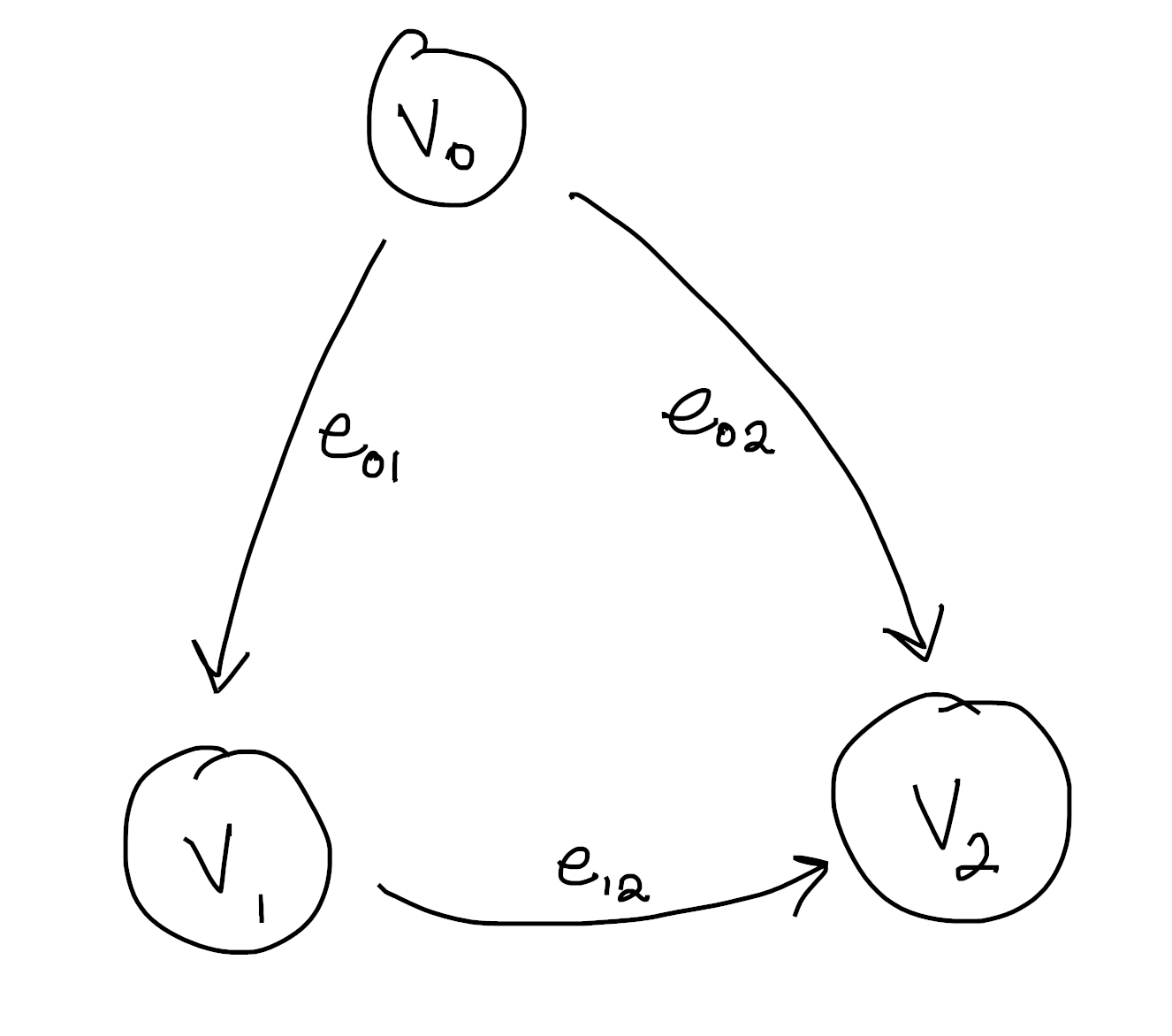
Notice the edges are always oriented from the smaller vertex to the bigger one. This is not an accident, and keeping a consistent choice of orientation is important for what follows. The simplest approach is to order your vertices, then follow the convention of $small \to large$

Now our problem will be to “integrate” a function defined on the edges to one defined on the vertices. What do I mean by this? Let’s see some concrete examples:

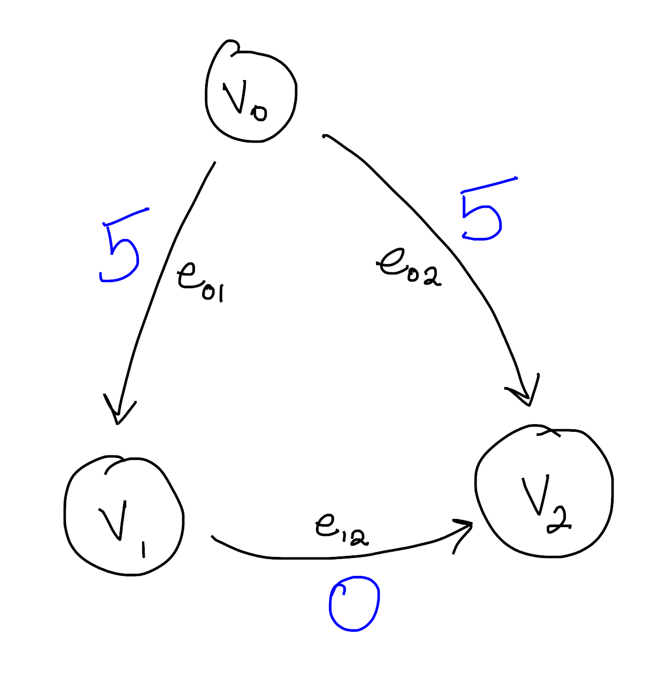
Here we see a function defined on the edges. Indeed, we could write this more formally as

\begin{aligned} f (e_{01}) & = 5 \\ f (e_{02}) & = 5 \\ f (e_{12}) & = 0 \end{aligned}

The goal now is to find a function on the vertices whose difference along each edge agrees with our function. This is what I mean when I say we’re “integrating” this edge function to the vertices. It’s not hard to see that the following works:

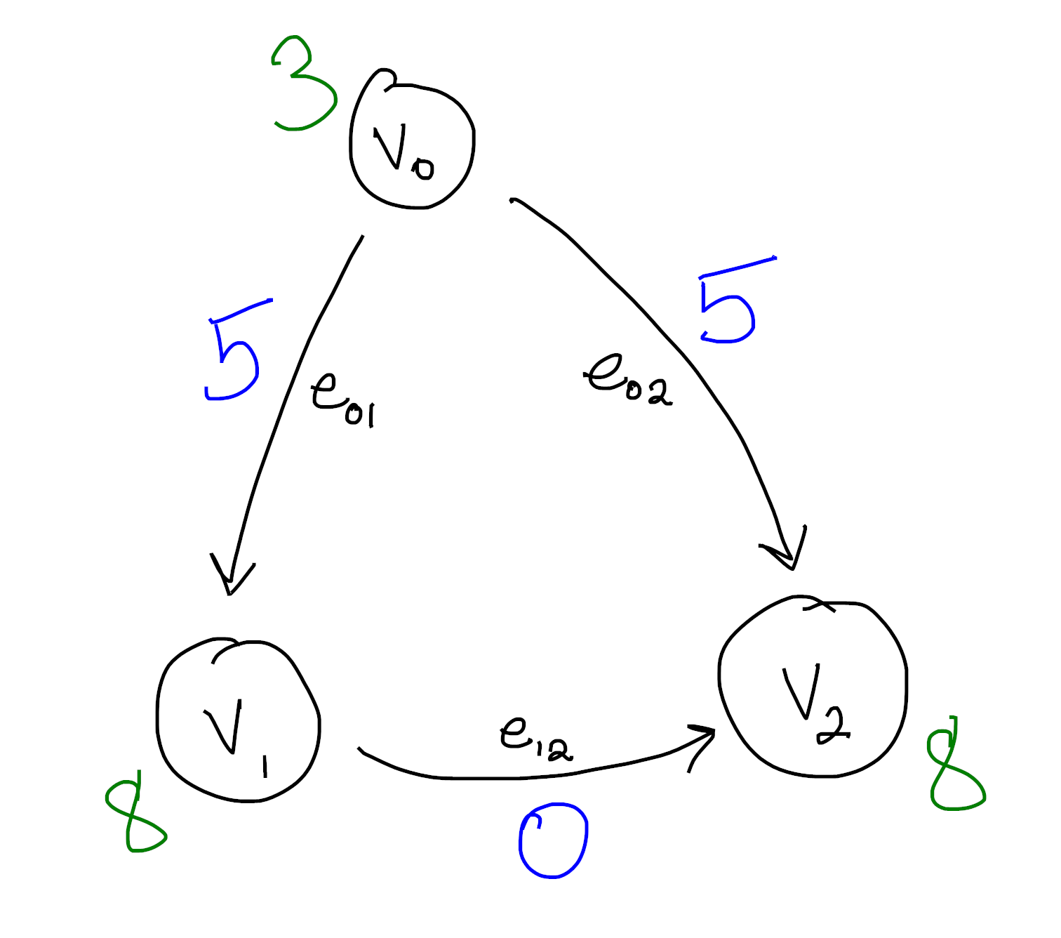
Again, if you like symbols, we can write this as

\begin{aligned} F (v_{0}) & = 3 \\ F (v_{1}) & = 8 \\ F (v_{2}) & = 8 \end{aligned}

Then we see for each edge $f (e_{i j}) = F (v_{j}) - F (v_{i})$ . This may seem like a weird problem to try and solve, but at least we solved it! Notice we pick up an arbitrary constant when we do this – We can set $v_{0} = C$ for any $C$ we want as long as $v_{1} = v_{2} = C + 5$ . This is one parallel with integration, and helps justify our language.

As some more justification, notice this obeys a kind of “fundamental theorem of calculus”: If you want to know the total edge values along some path, $\sum_{v_{k_{1}} \to v_{k_{2}} \to \dots \to v_{k_{n}}} f (e_{k_{i}, k_{i + 1}})$ , that turns out to be exactly $F (k_{n}) - F (k_{1})$ for some “antiderivative” $F$ of $f$ .

As a (fun?) exercise, you might try to formulate and prove an analogue of the other half of the fundamental theorem of calculus. That is, can you formulate a kind of “derivative” $d$ which takes functions on the vertices to functions on the edges? Once you have, can you show that differentiating an antideriavtive gets you your original function?

For (entirely imaginary) bonus points, you might try to come up with a parallel between edge functions of the form $d F$ (that is, edge functions which have an antiderivative) and conservative vector fields.

Let’s look at a different function now:

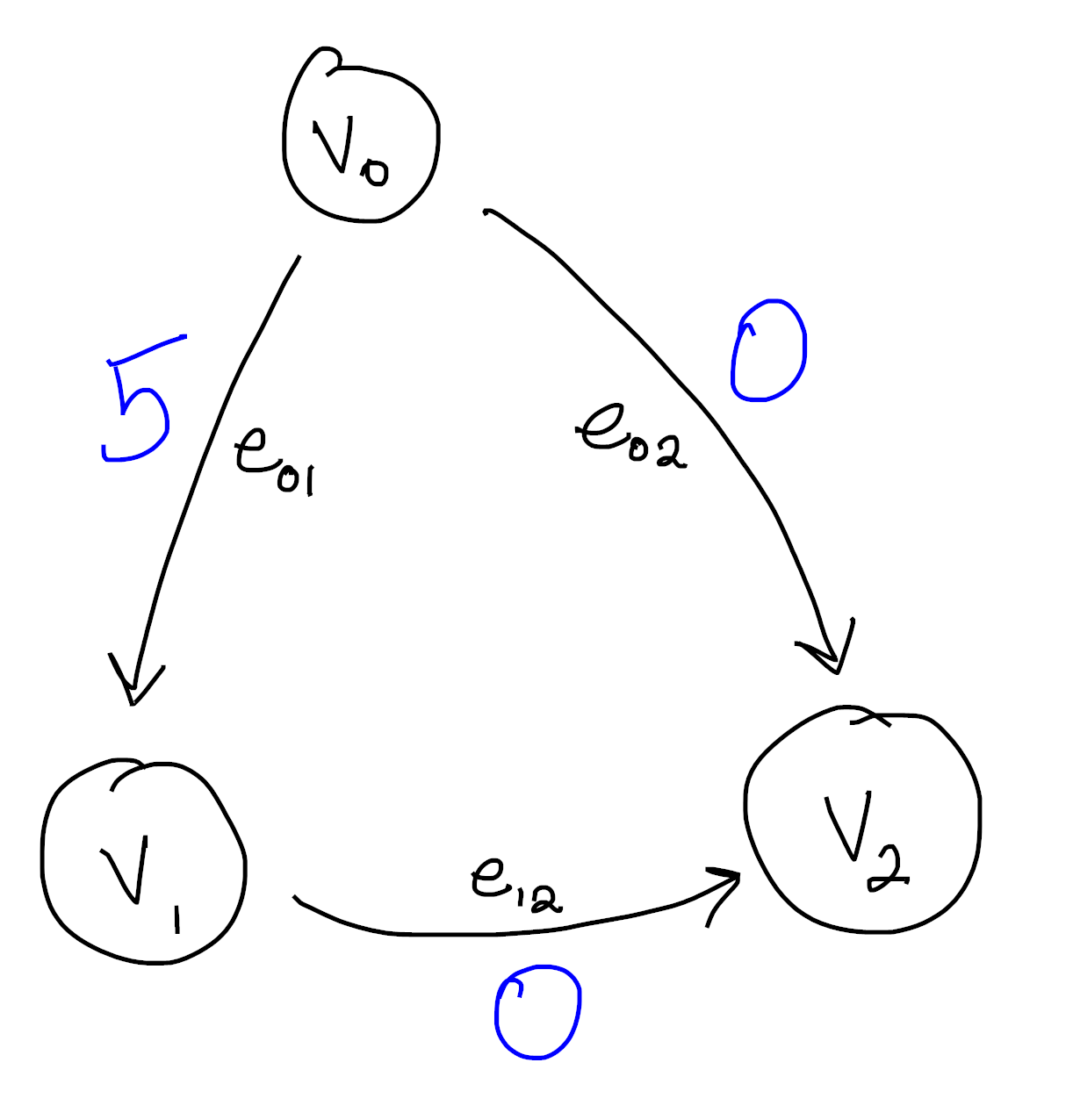
You can quickly convince yourself that no matter how hard you try, you can’t integrate this function. There is no antiderivative in the sense that no function on the vertices can possibly be compatible with our function on the edges.

After all, say we assign $v_{0}$ the value $C$ . Then $v_{1}$ is forced into the value $C + 5$ in order to agree with $e_{01}$ . But then because of $e_{12}$ we must set $v_{2} = C + 5$ as well, and uh oh! Our hand was forced at every step, but looking at $e_{02}$ we see were out of luck.

This should feel at least superficially similar to the $\sqrt{\cdot}$ example from earlier. At each step along the way, it’s easy to solve our problem: If you know what $F (v_{i})$ is, and you see an edge $v_{i} \to v_{j}$ , just assign $F (v_{j})$ to $F (v_{i}) + f (e_{i j})$ . The problem comes from making these choices consistently, which turns out to not always be possible!

As an aside, you can see that the problem comes from the fact that our graph has a cycle in it. Can you show that, on an acyclic graph, every edge function can be integrated to a function on the vertices?

We will soon see that the functions which can’t be integrated are (modulo an equivalence relation) exactly the cohomology classes. So the presence of a function which can’t be integrated means there must be a cycle in our graph, and it is in this sense that cohomology “detects holes”.

This is entirely analogous to the fact that every (irrotational) vector field on a simply connected domain is conservative. It seems the presence of some “hole” is the reason some functions don’t have primitives.

Ok, so now we know what problem we’re trying to solve. When can we find an antiderivative for one of these edge functions? The machinery ends up being a bit complicated, but that’s in part because we’re working with graphs, which are one dimensional simplicial complexes. This exact same setup works for spaces of arbitrary dimension, so it makes sense that it would feel a bit overpowered for our comparatively tiny example.

First things first, we look at the free abelian groups generated by our $n$ -dimensional cells. For us, we only have $0$ -dimensional vertices and $1$ -dimensional edges. So we have to consider two groups:

Z E and Z V

For the example from before, that means

Z {e_{01}, e_{12}, e_{02}} and Z {v_{0}, v_{1}, v_{2}}

which are both isomorphic to $Z \oplus Z \oplus Z$ .

Second things second. We want to connect these two groups together in a way that reflects the combinatorial structure. We do this with the Boundary Map $\partial : Z E \to Z V$ . This map takes an edge to its “boundary”, so $\partial e_{01} = v_{1} - v_{0}$ . Since we have a basis floating around anyways, it’s convenient to represent this map by a matrix:

\partial = (\begin{matrix} - 1 & 0 & - 1 \\ 1 & - 1 & 0 \\ 0 & 1 & 1 \end{matrix})

So for instance,

\partial e_{01} = (\begin{matrix} - 1 & 0 & - 1 \\ 1 & - 1 & 0 \\ 0 & 1 & 1 \end{matrix}) (\begin{matrix} 1 \\ 0 \\ 0 \end{matrix}) = (\begin{matrix} - 1 \\ 1 \\ 0 \end{matrix}) = v_{1} - v_{0}

Now our groups assemble into a Chain Complex:

\dots \to 0 \to 0 \to Z E \overset{\partial}{⟶} Z V

The extra groups $0$ correspond to higher dimensional simplices that aren’t present for us. If we filled in our cycle with a $2$ -dimensional triangular face, then we would have an extra group $Z F$ and an extra map (which is also called $\partial$ , rather abusively) from $Z F \to Z E$ which takes a face to its boundary (this might also help explain the term “boundary”). Then if we had a “cycle” of faces, we could fill them in with a (solid) tetrahedron. So we would have a new group $Z T$ , equipped with a map $\partial : Z T \to Z F$ taking each tetrahedron to its boundary of faces. Of course, this goes on and on into higher and higher dimensions⁵.

There’s actually a technical condition to be a chain complex that’s automatically satisfied for us because our chain only has one interesting “link”. Given an $n + 2$ -dimensional simplex $σ$ , we need to know that $\partial \partial σ = 0$ . I won’t say much more about it now, but I might write a blog post giving examples of higher-dimensional simplicial cohomology at some point. When that happens, we’ll have no choice but to go into more detail.

As a quick exercise:

What is the boundary $\partial (e_{01} + e_{12})$ ? What, intuitively, does $e_{01} + e_{12}$ represent? Does it make sense why the boundary of this figure should be what it is?

What about $\partial (e_{01} + e_{12} - e_{02})$ ? Again, what does $e_{01} + e_{12} - e_{02}$ represent? Does it make sense why the boundary of this figure should be what it is?

So we know that elements of $Z E$ (resp. $Z V$ ) represent (linear combinations of) edges (resp. vertices). Of course, we want to look at functions defined on the edges and vertices. So our next step is to dualize this chain:

\dots \leftarrow Hom (0, R) \leftarrow Hom (0, R) \leftarrow Hom (Z E, R) \overset{\partial^{T}}{⟵} Hom (Z V, R)

We’re now looking at all (linear) functions from $Z E \to R$ (resp. $Z V \to R$ ). By the universal property of free abelian groups, though, we know that the functions $Z E \to R$ correspond exactly to the functions $E \to R$ (extended linearly).

Moreover, our boundary operator $\partial$ has become a coboundary operator $\partial^{T}$ that points the other direction⁶. Here if $F : V \to R$ then we define $\partial^{T} f : E \to R$ by

(\partial^{T} F) (e) = F (\partial e)

Moreover, our notation $\partial^{T}$ is not misleading. $Hom (Z V, R)$ has a basis of characteristic functions

{χ_{v_{0}}, χ_{v_{1}}, χ_{v_{2}}}

where

χ_{v_{i}} (v_{j}) = {\begin{cases} 1 & i = j \\ 0 & i \neq j \end{cases}

Similarly $Hom (Z E, R)$ has a basis of characteristic functions, and it turns out that, with respect to these “dual bases”, the map $\partial^{T}$ is actually represented by the transpose of $\partial$ !

If you haven’t seen this before, you should convince yourself that it’s true. Remember that the transpose of a matrix has something to do with dualizing.

Moreover, you should check that a function $f$ on the edges is in the image of $\partial^{T}$ exactly when it can be integrated. Moreover, if $f = \partial^{T} F$ , then $F$ is an antiderivative for $f$ .

We’re in the home stretch! The second half of that box alludes to something important: A function $f$ can be integrated exactly when it is in the image of $\partial^{T}$ . With this in mind, we’re finally led to the definition of the cohomlogy group of our graph:

Since the only map $0 \to R$ is the trivial one, we can rewrite our complex as:

\dots \overset{0}{\leftarrow} 0 \overset{0}{\leftarrow} 0 \overset{0}{\leftarrow} Hom (Z E, R) \overset{\partial^{T}}{⟵} Hom (Z j, R)

Then we define⁷

H^{1} = \frac{Ker (\partial^{T} : Hom (Z E, R) \to 0)}{Im (\partial^{T} : Hom (Z V, R) \to Hom (Z E, R))}

Since there are no two dimensional faces, $\partial^{T} : Z E \to 0$ is the trivial map, and so its kernel is everything. In light of this, we see a slightly simpler definition of $H^{1}$ :

H^{1} = \frac{Hom (Z E, R)}{Im (\partial^{T} : Hom (Z V, R) \to Hom (Z E, R))}

This says the elements of $H^{1}$ are exactly the functions on edges, but we’ve quotiented out by all the functions that we can integrate to the vertices! So if we want to check if a function can be integrated, we just compute its cohomology class and check if it’s $0$ .

Moreover, the basis of $H^{1}$ as an $R$ -vector space give us a collection of “basic” non-integrable functions. Then every function on the edges can be written as an integrable one, plus some linear combination of the basic nonintegrable ones. This dramatically reduces the number of things we have to think about! From the point of view of integration, we only need to worry about the “good” functions (which admit antiderivatives) and (typically finitely many) “bad” functions which we can handle on a case-by-case basis.

If we put $0$ s to the right of $Z V$ as well as to the left of $Z E$ , we can also look at

H^{0} = \frac{Ker (\partial^{T} : Hom (Z V, R) \to Hom (Z E, R))}{Im (\partial^{T} : 0 \to Hom (Z V, R))} = Ker (\partial^{T} : Hom (Z V, R) \to Hom (Z E, R))

What is the dimension of $H^{0}$ in our example? What about for a graph with multiple connected components? In this sense, $H^{0}$ detects “ $0$ -dimensional holes”.

We’ve spent some time now talking about what cohomology is. But again, part of its power comes from how computable it is. Without the exposition, you can see it’s really a three step process:

Turn your combinatorial data into a chain complex by taking free abelian groups and writing down boundary matrices $\partial$ .
Dualize by hitting each group with $Hom (\cdot, R)$
Compute the kernels and images of $\partial^{T}$ , then take quotients.

Steps $1$ and $2$ should feel very good, and hopefully you’re aware that taking kernels and images of a linear map should be easy (even if I know I’m pretty rusty). It turns out computing a vector space quotient is also easy, though it’s much less widely taught. That doesn’t matter, though, since sage absolutely remmebers how to do it.

Since it’s so computable, and the best way to gain intuition for things is to work through examples, I’ve included some code to do just that!

Enter a description of a graph, and then try to figure out what you think the cohomology should be.

See if you can find geometric features of your graph which make the dimension obvious! If you want a bonus challenge, can you guess what the generators will be? Keep in mind there’s lots of generating sets, so you may get a different answer from what sage tells you even if you’re right.

You might also try to implement the algorithm we described yourself, at least for simple cases like graphs. You can then check yourself against the built in sage code below!

xxxxxxxxxx
 
# Write the edges in the box. 
# You can add isolated vertices by including 
# an 'edge' with only one vertex
@interact
def _(Simplices = input_box([["a"],["b","c"],["c","d"],["b","d"]], width=50), auto_update=False):
    show("The graph is:")
    S = SimplicialComplex(Simplices)
    show(S.graph()) # It looks like there's no builtin way to draw complexes...
    
    show("The chain complex is:")
    
    # we did it over the reals in the post,
    # but if we use the reals here, sage will
    # print 1.00000000000000 instead of 1...
    # so we're using the rationals instead
    C = S.chain_complex(base_ring=QQ)
​
    # mathjax uses its own font and I'm too lazy to change it
    # but it's not monospace, so the ascii_art looks silly
    # when we `show` it...
    # the solution is to print it instead, since I have
    # control over non-mathjax fonts. 
    # but printing doesn't flush the output buffer, so 
    # things show up in a silly order! 
    # we can fix this by manually flushing the buffer ourselves.
​
    # this means the cell complexes are going to be left-aligned, though
    # which we'll just have to deal with.
​
    print(ascii_art(C))
    sys.stdout.flush() 
​
    
    show("Which dualizes to:")
    
    Cdual = C.dual()
    print(ascii_art(Cdual))
    sys.stdout.flush()
    
    show("So the cohomology is:")
    
    # the cohomology of the original complex is
    # exactly the homology of the dual complex.
    H1 = Cdual.homology(deg=1,generators=True)
    show(QQ^(len(H1)))
    
    # Remember, the outputs here represent functions!
    # The entry in position i is the value that our
    # function assigns edge i
    show("With generators:")
    for g in H1:
        show(g[1].vector(1))

Help | Powered by SageMath

Messages

See, for instance, this wonderful series by Jeremy Kun, and even the wikipedia page. The basic idea is that homology groups correspond to “holes” in your space. These correspond to subsurfaces that aren’t “filled in”. That is, they aren’t the boundary of another subsurface. This is where the “boundary” terminology comes from. ↩
I know this is a link to simplicial homology, but there’s no good overview page (at least on the first page of google) for simplicial cohomology. It’s close enough, though, especially since we’re going to be spending a lot of time talking about simplicial cohomology in this post. ↩
If you’ve heard of sheaves before, this is also why we care about sheaves! They are the right “data structure” for keeping track of these “locally defined functions” that we’ve been talking about. ↩
We can tell we’re onto something important, though, because for nice spaces, all the different definitions secretly agree! Often when you have a topic that is very robust under changes of definition, it means you’re studying something real. We see a similar robustness in, for instance, the notion of computable function. There’s at least a half dozen useful definitions of computability, and it’s often useful to switch between them fluidly to solve a given problem. Analogously, we have a bunch of definitions of cohomology theories which are known to be equivalent in many contexts. It’s similarly useful to keep multiple in your head at once and use the one best suited to a given problem. ↩
For $\partial$ from edges to vertices, we know what our orientation should be (always subtract the low vertex from the high vertex), but it’s less clear what signs each of the edges bounding a triangle should receive… It’s even less clear what signs the faces bounding a tetrahedron should get! In fact, the issue of signs (and orientation in general) is a bit fussy. Once you pick a convention, though (for us, it’s high minus low), the orientation in higher dimensions is set in stone. You shouldn’t worry too much about the formulas for $\partial$ . What matters is the signs are chosen to make $\partial \partial σ = 0$ for every $n + 2$ -simplex $σ$ . This should make a certain amount of sense, as the boundary of a figure should not have its own boundary… Thats worth some meditation. ↩
Oftentimes you’ll see this written as $d$ in the literature, since it acts like a differential. Indeed in the case of De Rham Cohomology it literally is the derivative! ↩
In general, if we have a complex $\dots \overset{\partial_{n + 2}^{T}}{⟵} C^{n + 1} \overset{\partial_{n + 1}^{T}}{⟵} C^{n} \overset{\partial_{n}^{T}}{⟵} C^{n - 1} \overset{\partial_{n - 1}^{T}}{⟵} \dots$ The $n$ th cohomology group is $H^{n} = \frac{Ker (\partial_{n + 1}^{T} : C^{n} \to C^{n + 1})}{Im (\partial_{n}^{T} : C^{n - 1} \to C^{n})}$ Again, if I end up writing a follow-up post with higher dimensional examples, you’ll hear lots more about this. ↩