$L^p$ Spaces

02 Sep 2021 - Tags: analysis-qual-prep

On to day $2$ of qual prep boogaloo. Yesterday Tuesday¹ was all about measures and integrable functions. Today, then, let’s talk about spaces of integrable functions. It’s time for $L^p$ spaces!

Thankfully, this should be a comparatively short post, since $L^p$ spaces are already pretty concrete, and (at least in my mind) don’t need a ton of motivation. We want to integrate things, and $L^p$ spaces (for $p \lt \infty$) collect the functions which we can integrate.

The lower values of $p$, such as $p=1$, put emphasis on the decay of a function near $\infty$. The benefit we gain is that they place relatively little emphasis on singularities.

Conversely, large values of $p$, such as $p=\infty$, put little emphasis on the decay of a function, but are more sensitive to (potentially mild) singularities.

As an example, think of $\frac{e^{-x}}{\sqrt{x}}$:

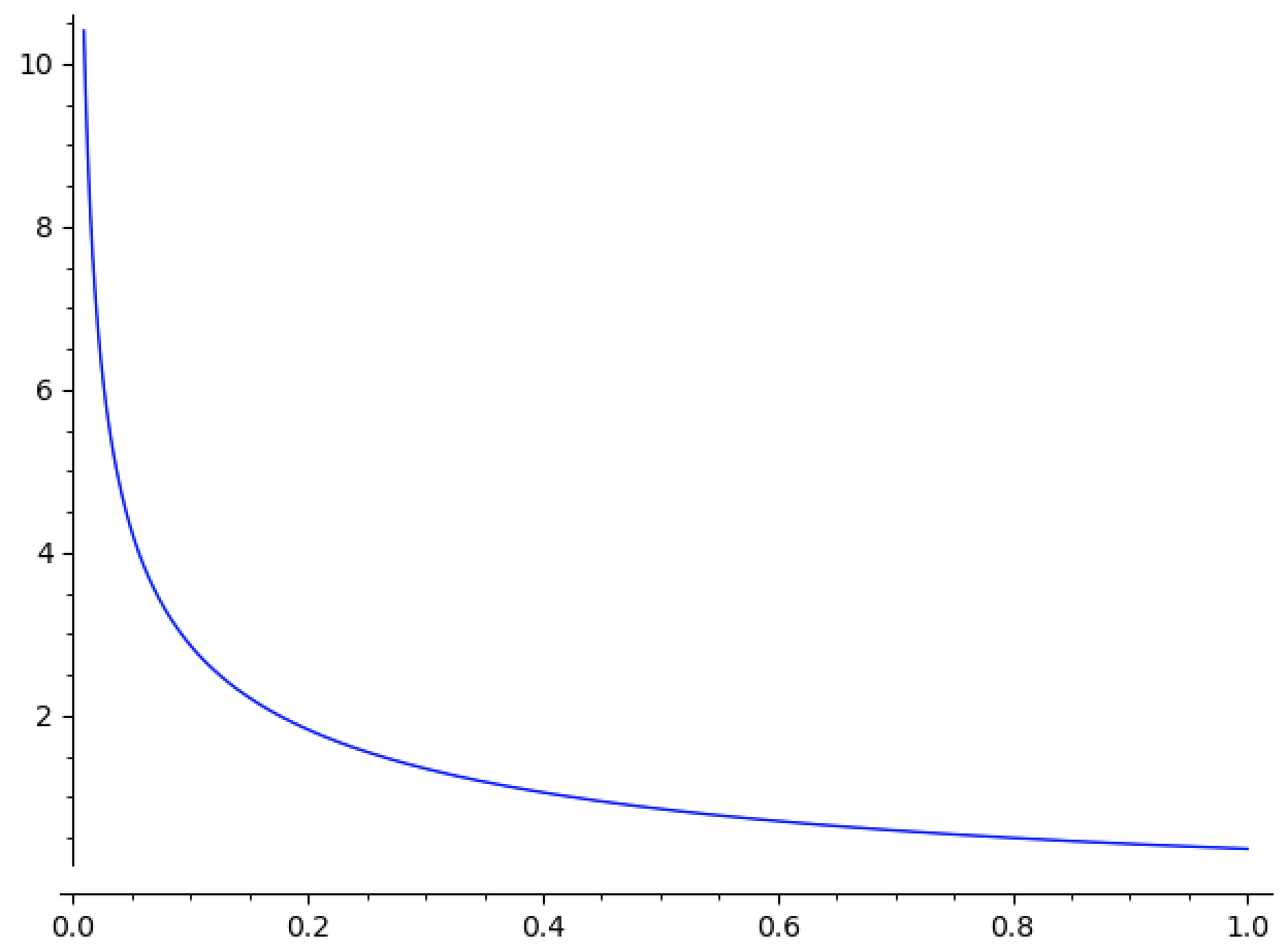
This has a singularity at $0$, but is still in $L^1(\mathbb{R})$ because it decays rapidly. This function is not in $L^2(\mathbb{R})$ (and certainly not in $L^\infty$), because its singularity is too sharp.

Conversely, consider the constant $1$ function, shown here for completeness more than anything else:

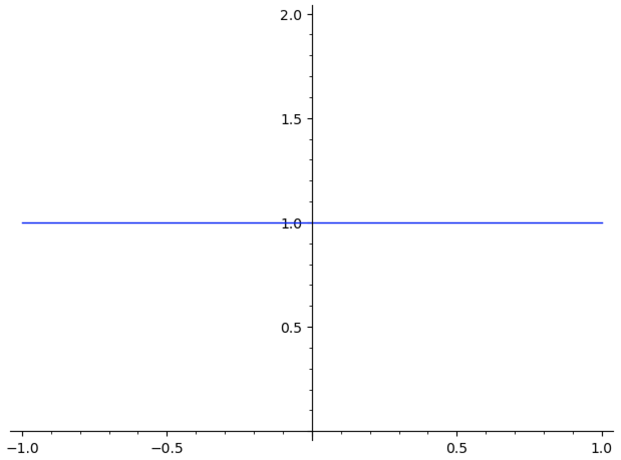
This function doesn’t decay at all, so is certainly not $L^1$. It turns out this function is only $L^\infty$, which doesn’t care at all about decay. It only cares about boundedness.

A less silly example might be $\chi_{[1,\infty)} \frac{1}{x}$:

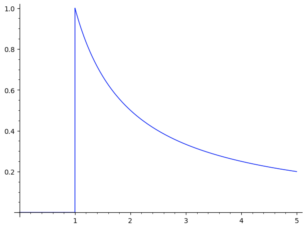
This function decays too slowly to be $L^1$, but it does decay quickly enough to be $L^2$.

The most important cases are $L^1$, $L^2$, and $L^\infty$, but there are reasons to care about other choices of $p$ as well. Psychologically, they let us interpolate between how much singularity we want to allow, versus how slowly we want to allow our functions to decay.

---

To start, let’s remind ourselves what $L^p$ spaces even are. We fix a set $X$ with a measure $\mu$. Then (for $1 \leq p \lt \infty$), we define the $p$-norm to be

\[\lVert f \rVert_p \triangleq \left ( \int |f|^p \ d \mu \right )^{1/p}\]

As is often the case, we need to treat $L^\infty$ specially. We write²

\[\lVert f \rVert_\infty \triangleq \inf \Big \{ M \ \Big | \ |f| \leq M \text{ a.e.} \Big \}\]

Now we can define (for $1 \leq p \leq \infty$)

\[L^p(X, \mu) \triangleq \bigg \{ f : X \to \mathbb{C} \ \bigg | \lVert f \rVert_p \lt \infty \bigg \}\]

As usual, we will consider two functions the same if they agree almost everywhere. We will also often write $L^p(X)$, $L^p(\mu)$, or even $L^p$ if the measure or space is clear from context.

It turns out $L^p(\mu)$ comes equipped with a ton of structure! The norm $\lVert f \rVert_p$ really is a norm³, and this norm makes $L^p(\mu)$ into a banach space (so we can talk about convergence without worry⁴).

Let’s see some important examples of $L^p$ spaces before we move on:

1. If $m$ is the lebesgue measure on $\mathbb{R}^n$, then $L^p(\mathbb{R}^n, m)$ is one of the most common examples used in practice. This forms the basis for a lot of intuition about $L^p$ spaces.

2. Sometimes $\mathbb{R}^n$ is too big. We might think of working with $L^p([a,b])$. Common choices are $[0,1]$ and $[0,2\pi]$.

3. Another important example is the circle $S^1$. The space $L^2(S^1)$ is the archetypal first example for fourier theory⁵.

4. An example in a different vein is $L^p(\mathbb{N})$ with the counting measure. This is often called $\ell^p$. Here our functions can be thought of as sequences of complex numbers, which makes this a particularly appealing setting for small examples. We’ll find $\ell^2$ extremely useful when we talk about hilbert spaces.

5. The counterpoint to example (3) is $L^p(\mathbb{Z})$, again with the counting measure. These are bi-infinite sequences of complex numbers, often written $\ell^p(\mathbb{Z})$, and these will be related to functions on the circle by means of the fourier transform.

---

One of the most important tools we have for proving properties about $L^p$ functions is the wide variety of dense subsets. If we want to prove something for all $L^p$ functions, we can start out by proving that thing for some subclass where we have more available tools, then argue by continuity that the result is actually true for all $L^p$ functions.

These sets of functions are dense in $L^p(\mathbb{R}^n)$ and $L^p([0,1])$, where $p \neq \infty$. More generally, they are true in $L^p(X,\mu)$ for radon measures on locally compact hausdorff spaces. See Rudin’s Real and Complex Analysis for more details.

• Simple Functions (with finite-measure support). That is, functions of the form \(\sum_{k=1}^n c_k \chi_{E_k}\). These are dense almost by definition⁶ and form the base for proving other, more exiting density results. After all, to show a class of functions is dense in $L^p$, it suffices to show it can approximate the simple functions. If we allow infinite measure support, then these functions are dense in $L^\infty$ as well.

• Continuous Functions (with compact support). Obviously these are great. We don’t always need the extra power of compact support, but it’s good to know it’s there!

These families of dense functions require a notion of differentiation. They’re definitely true in $\mathbb{R}^n$ and $[0,1]$, and I suspect they’re true over any manifold. I don’t have a reference on hand, though.

• Smooth Functions (with compact support). We love differentiation in this household.

• Schwarz Functions. As long as we’re discussing things that only work in $\mathbb{R}^n$, these are functions which are not only smooth, but which vanish more quickly than any polynomial, and all their derivatives vanish that quickly too. We’ll talk more about these in the post about fourier theory.

These families of functions also require some compactness condition (because we’re using the stone-weierstrass theorem).

• Polynomials. On $[0,1]$, we can approximate by polynomials

• Polynomials in $e^{ix}$. On $S^1$, we can approximate by “trigonometric polynomials”. This will be extremely important when we start talking about fourier theory.

There’s actually a kind of master theorem for density results in $L^p$ spaces ($p \neq \infty$), which takes some basic properties of a class of functions and tells you it’s dense. There are also generalizations of the theorems above to much more broad classes of measure spaces. For each of these results, see this pdf from Bruce Driver’s UCSD lecture notes.

Before we move on, these density results are one potential source of motivation for $L^1$. We’re obviously interested in continuous functions, and if we want to integrate things, the $L^1$ norm seems like a fairly reasonable metric to look at. The issue is that $L^1$ limits of continuous functions don’t need to be continuous! That is, $CX$ is not complete with respect to the $L^1$ norm. We like to know we can take limits with reckless abandon⁷, so we should take its completion. When we do this, we get exactly the $L^1$ functions.

This is one reason that $L^\infty$ behaves “pathologically” compared to the other $L^p$ spaces. When you take the completion of continuous functions with compact support in the $p$-norm for $p \lt \infty$, get get exactly $L^p$. However, when you take the completion in the $\infty$-norm, you get the functions vanishing at $\infty$. You might try to solve this by looking at the bounded continuous functions, rather than those of compact support⁸, but these already form a banach space! It seems that, unavoidably, $L^\infty$ has a bunch of extra stuff in it, and it’s this extra stuff that is responsible for many of the differences between $L^\infty$ and the other $L^p$ spaces.

---

Perhaps the most important inequality associated with $L^p$ spaces is Hölder’s inequality, which generalizes the Cauchy-Schwarz inequality.

Here we might think of $g$ as defining a functional $\phi_g$, where $\phi_g f \triangleq \int f g$. Then Hölder’s inequality says that (with the operator norm) $\lVert \phi_g \rVert \leq \lVert g \rVert_q$.

From this, one might ask if we actually have equality above. If you’re feeling particularly optimistic, you might even wonder if we can characterize which functionals in $(L^p)^*$ arise as $\phi_g$ for some $g \in L^q$.

Now for the magic part:

The proof of this fact actually goes through complex valued measures! If $\phi$ is a functional on $L^p$, then it’s not hard to see that $\nu E \triangleq \phi \chi_E$ is a (complex valued) measure! Moreover, if $E$ is $\mu$-null, then $\chi_E = 0$ a.e., and so $\nu E = \phi \chi_E = 0$. This means $\nu \ll \mu$, and so by radon-nikodym $\nu = \mu_g$ for some function $g$. Now some simple bookkeeping is all we need to do to show that $g \in L^q$ and $\phi f = \int fg$.

Notice this means that for $1 \lt p \lt \infty$ we have

\[(L^p)^{**} = (L^q)^* = L^p\]

so $L^p$ is reflexive. It’s still not entirely obvious to me why reflexive spaces are as interesting as they are. It’s obviously a natural question (and a fairly algebraic one¹¹), and it gives you quite a bit of bonus information (see here, for instance). I suspect that I’ll come to appreciate it more as I do more functional analysis¹². At the very least, it’s nice to have a full characterization of the dual space, and it’s satisfying to get back where you started when you dualize twice.

---

Frequently one has a function $f \in L^p$, which we would like to know is in $L^q$. More generally, we would like to relate functions in $L^p$ to functions in $L^q$ with $q$ on either side of $p$.

For instance, when doing fourier analysis, our hilbert space techniques only work for $L^2(S^1)$ functions, which get mapped by the fourier transform isometrically onto $\ell^2(\mathbb Z)$. However, we can show that $\ell^1(\mathbb Z) \subseteq \ell^2(\mathbb Z)$, and thus we see that if $f$ is $L^1(S^1)$ and $\hat{f}$ is $\ell^1(\mathbb Z)$, then the results (which we’ll talk about soon) still hold.

With that said, here are the main theorems for useful inclusions:

In fact, both of the above statements are equivalences. So going down is allowed if and only if $X$ has finite measure, and going up is allowed if and only if $X$ has subsets of minimal measure¹³.

Notice how these line up with the singularity/rapid decay tradeoff we mentioned earlier. If $X$ has finite measure, then (intuitively) there’s no “infinity” to worry about decaying towards. So the decay penalization is irrelevant, and we get an inclusion of “lower singularity” functions into “higher singularity” functions with no further qualifications¹⁴.

Conversely, if there are sets of minimal measure, then (intuitively) any singularity on one of your atoms can’t be avoided, and we get the inclusion of “rapidly decaying” functions into “slowly decaying” functions with no further qualifications¹⁵.

Of course, once we know that, say $L^2([0,1]) \subseteq L^1([0,1])$, it’s natural to ask “how many $L^1$ functions are actually $L^2$?”. The answer is “almost none”!

It turns out that $L^2([0,1])$ is meagre in $L^1([0,1])$. This is a topological notion of “smallness” which is roughly akin to being a nullset¹⁶. This is a cute application of the baire category theorem, which is the topic of an upcoming blog post.

We also have interpolation functions which, if $p \lt q \lt r$, lets us relate $L^q$ functions to those on either side.

---

Alright, that was another huge information dump! This post felt less like a motivated tour through $L^p$ functions and more like a copy of a study guide, haha. I think that’s reasonable, though, since in my experience $L^p$ functions are pretty motivated by themselves. I’m mainly writing this so that when I talk about Banach spaces soon we’ll have all these examples to draw from. Plus, selfishly, it was nice to organize all this information while planning out this post.

I’ve learned from my mistakes, and I’m not going to try and give a concrete date for the next post. All I’ll say is: See you soon ^_^

---