Hilbert Spaces

15 Sep 2021 - Tags: analysis-qual-prep

Hilbert Spaces are banach spaces whose norms come from an inner product. This is fantastic, because inner product spaces are a very minimal amount of structure for the amount of geometry they buy us. Beacuse of the new geoemtric structure, many of the pathologies of banach spaces are absent from the theory of hilbert spaces, and the rigidity of the category of hilbert spaces (there is a complete cardinal invariant describing hilbert spaces up to isometric isomorphism) makes it extremely easy to make an abstract hilbert space concrete. Moreover, this “concretization” is exactly the genesis of the fourier transform!

With that introduction out of the way, let’s get to it!

---

First, a word on conventions. I’ll be working with the inner product $\langle x,y \rangle$ which is linear in the second slot, and conjugate linear in the first. This is often called the “physicist” notation, but I have a reason for it:

Since we write function application on the left², it makes sense for the associated functional $\langle x, \cdot \rangle$ to also be “on the left”. With the standard “mathematician” convention, we instead have the linear map $\langle \cdot, y \rangle$ which acts on $x$ “on the right” by $x \mapsto \langle x, y \rangle$.

Obviously this doesn’t matter at all, but I feel the need to draw attention to it³.

There are two key examples of hilbert spaces:

• $L^2(X,\mu)$ is a hilbert space, with the inner product

  \[\langle f, g \rangle \triangleq \int \overline{f} g \ d\mu\]

• A special case of the above, if $A$ is any set and $\#$ is the counting measure, then $\ell^2(A) = L^2(A, \#)$ is a hilbert space with the inner product

  \[\langle (x_\alpha), (y_\alpha) \rangle \triangleq \sum \overline{x_\alpha} y_\alpha\]

In fact, as we will see, every hilbert space is isometrically isomorphic to some $\ell^2(A)$, and just as we can distinguish vector spaces by the cardinality of their basis, we can distinguish hilbert spaces by the cardinality of their “hilbert basis”.

First, though, why should we care about inner products? How much extra structure does it really buy us? The answer is: lots!

As is so often the case in mathematics, theorems in a concrete setting become definitions in a more general setting, and once we do this much of the intuition for the concrete setting can be carried over. For us, then, let’s see what we can do with inner products.

---

First, it’s worth remembering that an inner product defines a norm

\[\lVert f \rVert \triangleq \sqrt{\langle f, f \rangle}\]

so every inner product preserving function also preserves the norm.

It turns out we can go the other way as well, and the polarization identity lets us write the inner product in terms of the norm⁴. This is fantastic, as it means any norm preserving function automatically preserves the inner product!

We can also define the angle between to vectors by

\[\cos \theta \triangleq \frac{\langle f, g \rangle}{\lVert f \rVert \lVert g \rVert}\]

and when $\theta = \pm \frac{\pi}{2}$ (that is, when $\langle f, g \rangle = 0$) we say that $f$ and $g$ are orthogonal, written $f \perp g$.

Of course, once we have orthogonality, we have a famous theorem from antiquity:

Once we have orthogonality, we also have the notion of orthogonal complements. You might remember from the finite dimensional setting that there’s (a priori) no distinguished complement to a subspace. For instance, any two distinct $1$-dimensional subspaces are complements in $\mathbb{R}^2$. But if we decomposed $\mathbb{R}^2$ as a direct sum of the subsaces shown below, we would likely feel there’s a “better choice” of complement for the orange subspace:

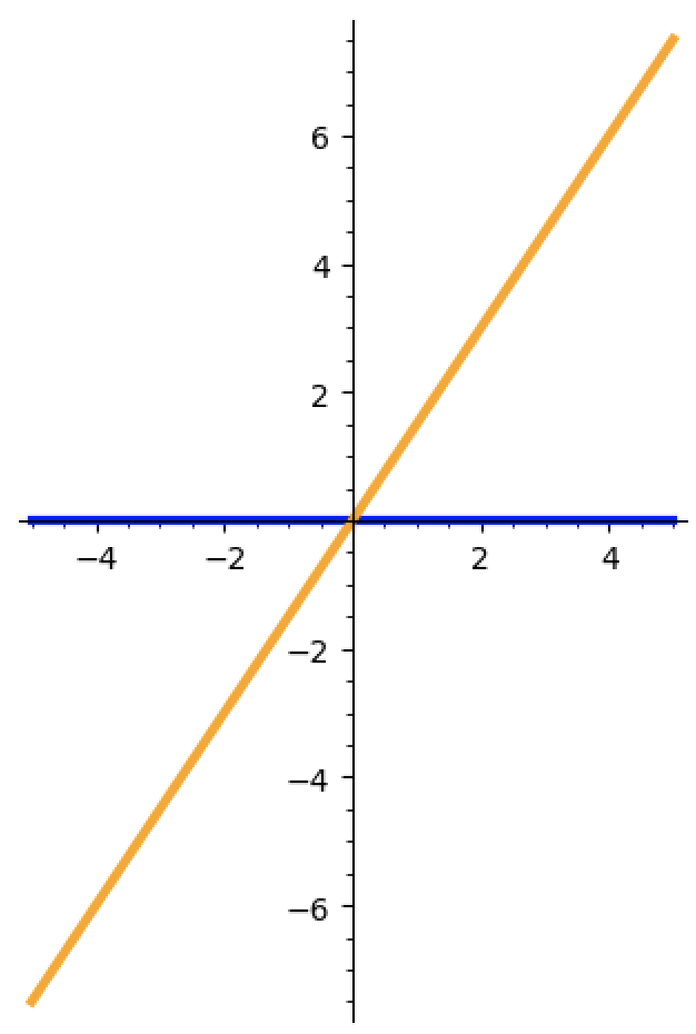
The blue subspace is one of many complements of the orange, so why should we choose it over anything else? Instead, we can use the inner product (in particular the notion of orthogonality) to choose a canonical complement:

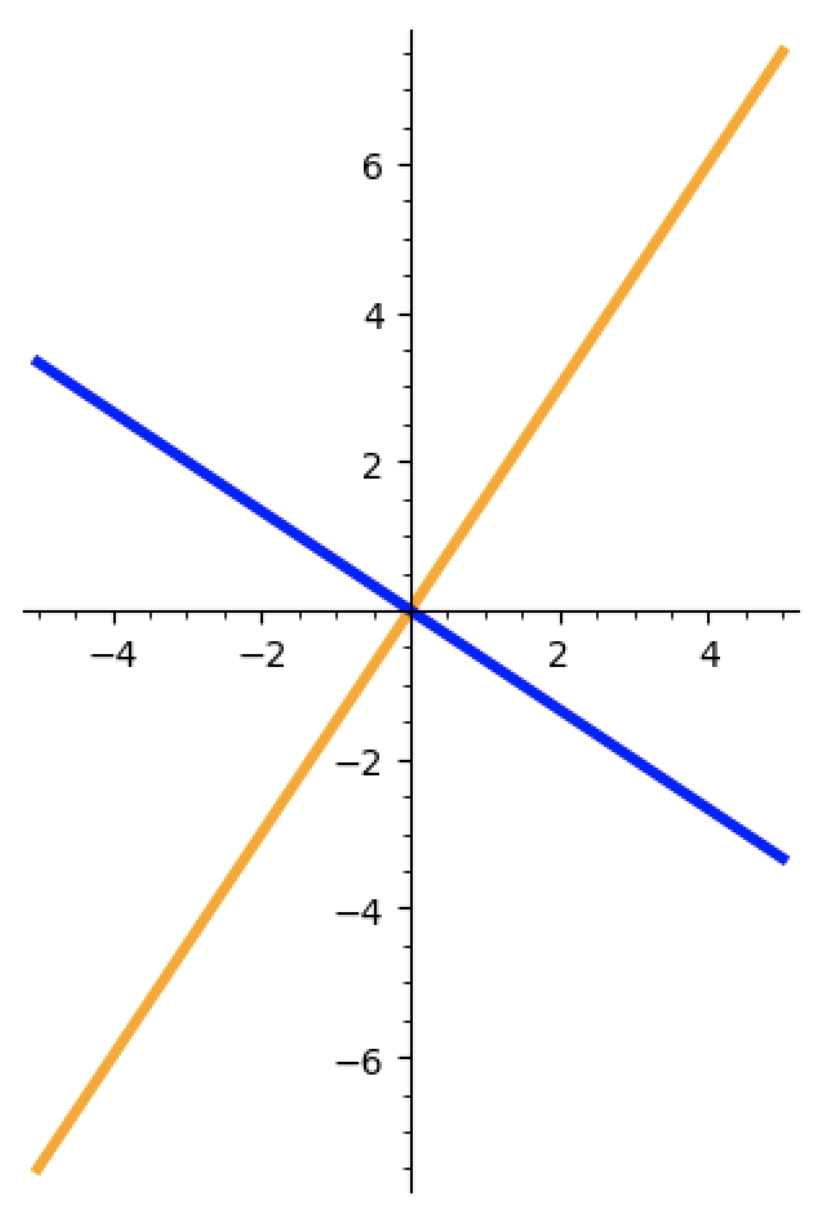
Why is this complement canonical? Because it is the unique complement so that every blue vector is orthogonal to every orange vector.

In the banach space setting (where we don’t have access to an inner product) recall there are subspaces which have no complement. In the hilbert space setting this problem vanishes – the orthogonal complement always exists, and is a complement⁵!

You might also remember from the finite case that we can find particuarly nice bases for inner product spaces (called orthonormal bases). It’s then natural to ask if there’s an analytic extension of this concept to the hilbert space setting.

The answer, of course, is “yes”:

These conditions are very foundational to hilbert space theory, and are worth remembering. The way that I like to remember is

In fact, one can show that the size of a hilbert basis is a complete invariant for hilbert spaces. That is, any two hilbert bases for $\mathcal{H}$ have the same cardinality (often called the Hilbert Dimension), and $\mathcal{H}_1 \cong \mathcal{H}_2$ if and only if they have the same hilbert dimension⁷.

---

That’s a lot of information about hilbert spaces in the abstract. But why should we care about any of this? Let’s see how to solve some problems using this machinery!

Let’s work with $L^2(S^1)$, the hilbert space of square-integrable functions on the unit circle. Classically, we would extend these to be periodic functions on $\mathbb{R}$, but that turns out to be the wrong point of view⁸.

A hilbert space is separable if and only if it has a countable hilbert basis. This is nice since most hilbert spaces arising in practice (including $L^2(S^1)$) are separable, so we can work with a countable sum (even though the theorem is true in more generality). For us, we note that \(\{ e^{inx} \}_{n \in \mathbb{Z}}\) is a hilbert basis for $L^2(S^1)$, sj we would expect periodic functions to decompose into an infinite sum of these basic functions.

Historically, it was a very important problem to understand the convergence of “fourier series”. That is, if we define

\[\hat{f}(n) \triangleq \int e^{-inx} f\]

(which we, with the benefit of hindsight, recognize as $\langle e^{inx}, f \rangle$)

when is it the case that we can recover $f$ as the sum $\displaystyle \sum_{-\infty}^\infty \hat{f}(n) e^{inx}$? That is, as the $n \to \infty$ limit of the partial fourier series

\[S_n f \triangleq \sum_{-n}^n \hat{f}(n) e^{inx}\]

In particular, for “nice” functions $f$, is it the case that $\displaystyle \lim_{n \to \infty} S_n f(x) \to f(x)$ pointwise? If not, is there some sense in which $S_n f \to f$?

This problem was fundamental for hundreds of years, with Fourier publishing his treatise on the theory of heat in $1822$, and there are textbooks written as recently as $1957$ which says it is unknown whether the fourier coefficients of a continuous function has to converge at even one point! See the historical survey here for more information, as well as the full course notes here by the same author.

The language of $L^p$ and Hilbert spaces wasn’t developed until the $1910$s, and they are integral (pun intended) in phrasing the solution of the fourier series convergence problem (Carleson’s Theorem).

Carleson’s theorem is famously hard to prove, be we can get a partial solution for free using the theory of hilbert spaces!

This is exactly the “density” part of the equivalence above! With some work, one can show that $S_n f \to f$ in the $L^p$ norm for any $p \neq 1, \infty$⁹.

Hilbert spaces are also useful in the world of ergodic theory. Say we have a function $T$ from some space $X$ to itself, which we should consider as describing how $X$ evolves over one time-step. One might expect that if we average the position of a point $x$ over time, we should converge on a fixed point of the transformation¹⁰.

A result in hilbert space theory tells us we aren’t off base!

This gives us the Mean Ergodic Theorem as a corollary!

---

Alright! We’ve seen some of the foundational results in hilbert space theory, and it’s worth remembering our techniques from the banach space world still apply. Hilbert spaces are very common in analysis, with application in PDEs, Ergodic Theory, Fourier Theory and more. The ability to basically do algebra as we would expect, and leverage our geometric intuition, is extremely useful in practice.

Next time, we’ll give a quick tour of applications of the Baire Category Theorem, and then it’s on to the Fourier Transform on $\mathbb{R}$!

The qual is a week from today, but I’m starting to feel better about the material. This has been super useful in organizing my thoughts, and if I’m lucky, you all might find them helpful as well.

If you have been, thanks for reading! And I’ll see you next time ^_^.

---