Some Questions about the Mathematics of Hitomezashi

19 Dec 2021 - Tags: sage

A little while ago I made a post with some sage code that makes pretty pictures based on a certain Japanese stitching based off of Hitomezashi Sashiko. It’s fun to play with, and I love making pretty pictures, but it also raises some interesting combinatorial questions! Questions which, unfortunately, I’m not sure how to answer. This post is about some partial progress that I’ve made, and also shows how I’ve been using sage to develop conjectures for these problems. I’ll end with the statement of a few of these conjectures, and if I’m lucky some readers will have ideas for attacking these problems!

First things first, let’s give a slightly more precise definition of the objects of interest. To each pair of binary strings $s_{1}$ and $s_{2}$ , say of lengths $n_{1}$ and $n_{2}$ , we’re going to associate a Hitomezashi Graph as follows:

We have vertices $[n_{1}] \times [n_{2}]$ , and we have edge relations as follows:

$(x, y) \sim (x + 1, y)$ if and only if $y ≢ s_{1} [x + 1] (\mod 2)$
$(x, y) \sim (x, y + 1)$ if and only if $x ≢ s_{2} [y + 1] (\mod 2)$

Intuitively, we alternate putting a wall between adjacent cells of a grid. A $0$ or a $1$ in position $k$ tells us whether we start with or without a wall.

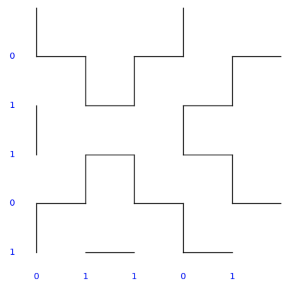
As a small example, let’s consider the strings

$s_{1} = 01101$
$s_{2} = 10110$

Then the resulting stitch pattern (as drawn by the code in the previous post) is

and the graph looks like this (overlayed on it):

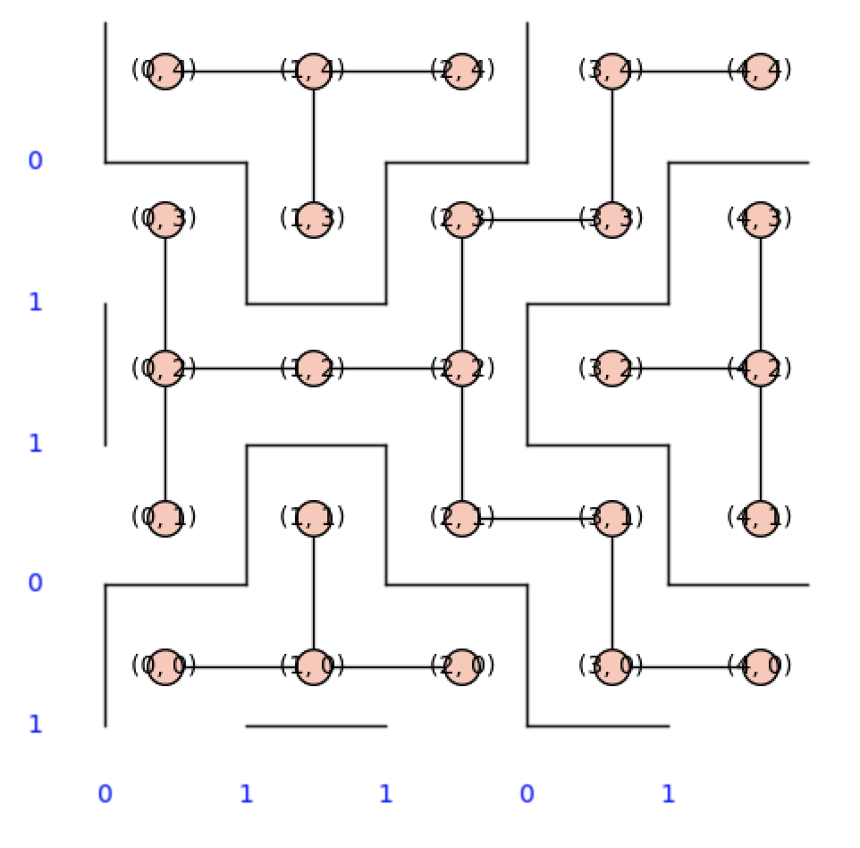
(Notice the “regions” in the picture are exactly connected components of the graph)

Now there’s a lot of of questions we can ask about these pictures. Let’s build a larger one to make things a bit more obvious:

Say $s_{1} = 11010100110111000000001$ and $s_{2} = 01001010110111110011110000110000$ .

then our picture looks like this:

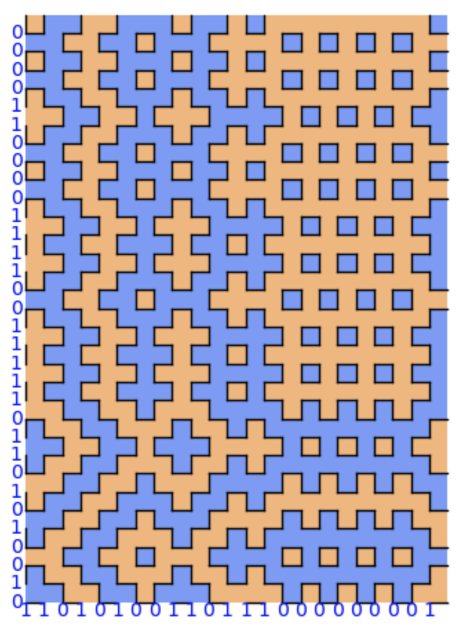
and already there’s some obvious questions to ask.

How many $1 \times 1$ squares do we expect to get? What about other patterns, like the plus signs?
How many regions do we expect to get in total? And how big do we expect the regions to be?

There are other natural questions as well, but these are interesting to me because I can solve them, and because I can’t solve them (respectively).

You should play around with making your own hitomezashi pictures, and try to come up with your own questions about them!

Feel free to leave any conjectures or work of your own in the comments here ^_^

Let’s start with the expected number of $1 \times 1$ tiles. This is actually a super cute problem, and could easily have been 251 homework at CMU. If you want to work it out for yourself, now’s the time! Otherwise, let’s see how to do it together:

The probability that any given square $(x, y)$ is a singleton tile is the probabillity that there are walls at $x$ , $x + 1$ , $y$ , and $y + 1$ . Of course, there’s a $50 %$ chance of having a wall in any predetermined position, So the odds of getting all $4$ of our walls in the right spot is $2^{- 4}$ .

Now (using linearity of expectation) we compute

\begin{aligned} E [# of 1 \times 1 cells] & = E [\sum_{(x, y)} 𝟙_{(x, y) is a 1 \times 1 cell}] \\ = \sum_{(x, y)} E [𝟙_{(x, y) is a 1 \times 1 cell}] \\ = \sum_{(x, y)} P [(x, y) is a 1 \times 1 cell] \\ = \sum_{(x, y)} \frac{1}{16} \\ = \frac{n_{1} n_{2}}{16} \end{aligned}

Of course, we can also code this up and check! Here is some code that

makes and draws Hitomezashi graphs
builds a random graph of size $n^{2}$ , and gets some information about it
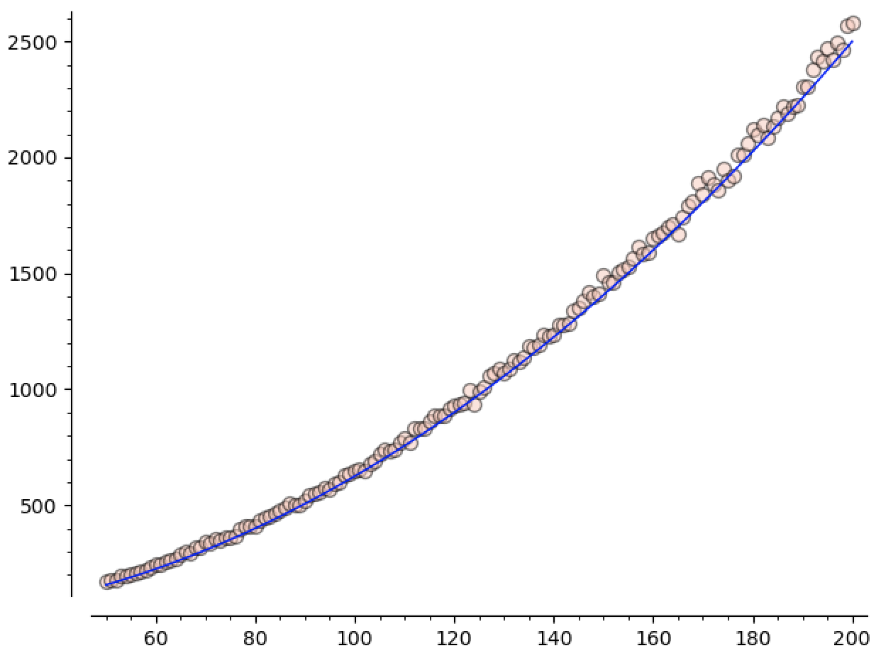
runs this 50 times for boards of size 50 to 200, keeping track of the average number of singletons for each choice of $n$ .

xxxxxxxxxx
 
def mkHitomezashi(s1,s2):
  """
  Make a hitomezashi graph based on @s1 and @s2
  """
  m = len(s1)
  n = len(s2)
​
  vs = [(x,y) for x in range(m) for y in range(n)]
​
  es = []
  for x in range(m):
    for y in range(n):
      if x+1 < m and y%2 != s1[x+1]:
        es += [((x,y),(x+1,y))]
      if y+1 < n and x%2 != s2[y+1]:
        es += [((x,y),(x,y+1))]
​
  return Graph([vs,es], format='vertices_and_edges')
​
​
def drawHitomezashi(G):
  """
  Draw the hitomezashi graph using the veretex names as positions
  """
  pos = {}
  for v in G.vertices():
    pos[v] = v
  
  return G.graphplot(pos=pos)
​
​
def runTest(n,p=None,q=None):
  """
  Build a random @n by @n graph, and get some stats
​
  @p is the probability of getting a 0 in the rows
  @q is the probability of getting a 0 in the columns
  """
​
  if p == None:
    p = 0.5
  if q == None:
    q = 0.5
​
  s1 = [int(random() < p) for blah in range(n)]
  s2 = [int(random() < q) for blah in range(n)]
​
  G = mkHitomezashi(s1,s2)
​
  # This is a list of the sizes of the connected components, 
  # in decreasing order of size.
  return G.connected_components_sizes()
​
​
def getNumSingletons(n, N, p=None, q=None):
  """
  get the mean and std dev number of singletons
​
  run @N many tests on graphs of size @n
  """
​
  numSingletons = []
  for _ in range(N):
    ccSizes = runTest(n,p,q)
    numSingletons += [ccSizes.count(1)]
​
  return (mean(numSingletons), sqrt(variance(numSingletons)))
​
​
def plotNumSingletons(n0,n1,N=None,p=None,q=None):
  """
  Run @N trials on sizes @n0 to @n1 and plot/return the data
  """
  if N == None:
    N = 100
​
  data = []
  for n in range(n0,n1+1):
    print(n)
    (avg,std) = getNumSingletons(n,N,p,q)
    data += [(n, avg.n())]
​
  show(scatter_plot(data) + plot(x^2/16, x, n0,n 1))
  return data
​
# plotNumSingletons(50,200,50)

Here you can see the data plotted against $x^{2} / 16$ . I think it basically speaks for itself:

Of course, we can do a similar analysis to see that there are going to be $Θ (n^{2})$ many copies of any fixed pattern, in expectation. Moreover, if we have a pattern in mind, we can compute the leading coefficient implicit in this big-theta.

As a (fun?) exercise, how many plus-shapes do we expect to get in a random $n \times n$ Hitomezashi graph?

Keep in mind that the existence of certain walls will no longer be independent.

Now let’s move on to the number of regions, and the largest region size.

We just computed that there’s $Θ (n^{2})$ many singleton tiles, and obviously there can’t be more than $n^{2}$ regions in total! So we actually know the asymptotic behavior of the number of regions too. This is slightly unsatisfying, though. It would be nice to know what the leading coefficient is. It’s clear that lots of our regions come from $1 \times 1$ tiles, so we would expect the number of regions to be not much bigger than $n^{2} / 16$ … But precisely how much bigger do we expect it to be?

Again, we can write some code to test this out:

xxxxxxxxxx
 
def getNumCCs(n, N, p=None, q=None):
  """
  get the mean and std dev number of CC
  (connected components)
​
  run @N many tests on graphs of size @n
  """
​
  numCCs = []
  for _ in range(N):
    ccSizes = runTest(n,p,q)
    numCCs += [len(ccSizes)]
​
  return (mean(numCCs), sqrt(variance(numCCs)))
​
​
def plotNumCCs(n0, n1, N=None, p=None, q=None):
  """
  Run @N trials on sizes @n0 to @n1 and plot/return the data
  """
​
  if N == None:
    N = 100
​
  data = []
  for n in range(n0, n1+1):
    print(n)
    (avg,std) = getNumCCs(n,N,p,q)
    data += [(n, avg.n())]
  
  show(scatter_plot(data))
  return data
​
# CCData = plotNumCCs(50,200,50)

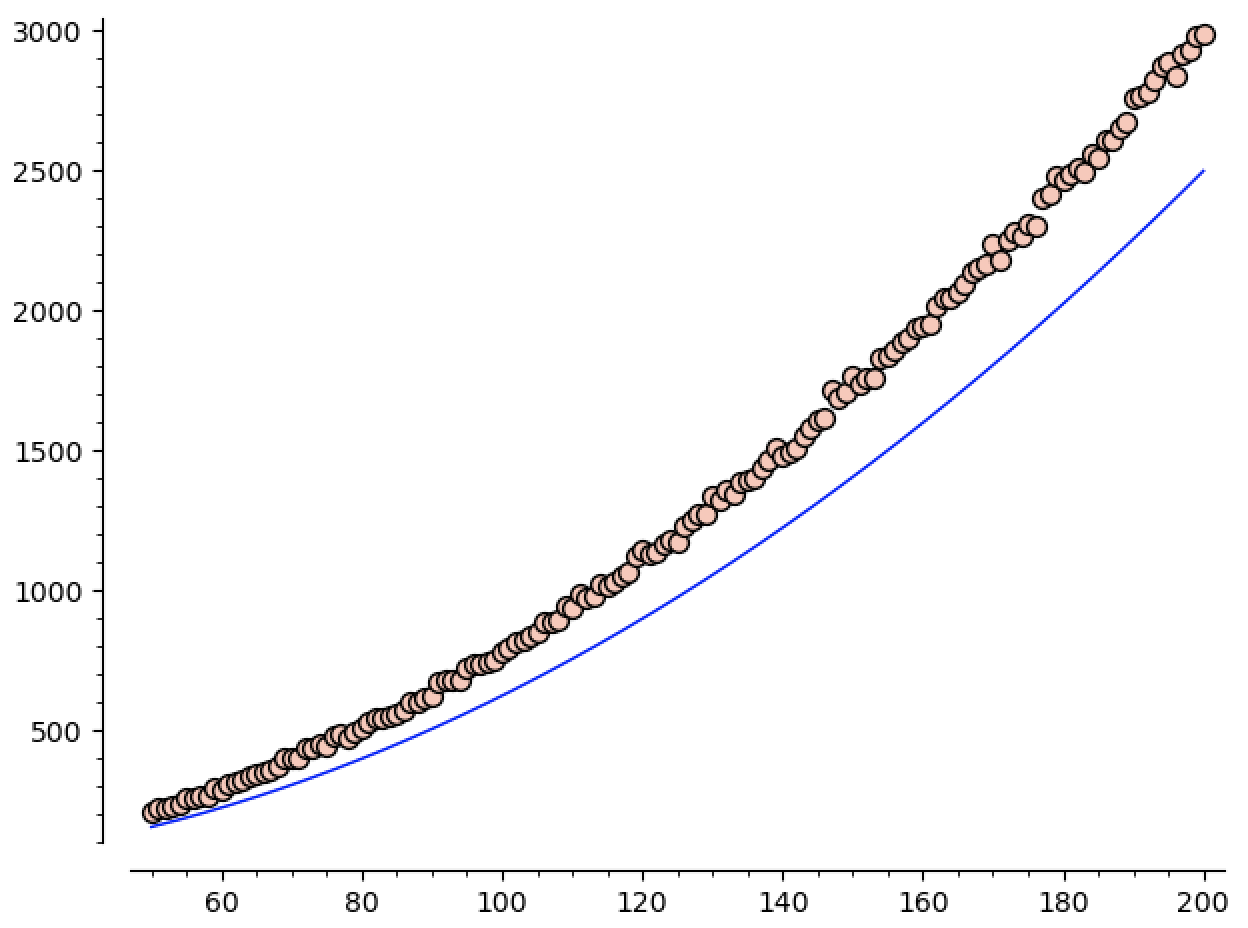
Here you can see the number of regions plotted against $x^{2} / 16$ . It’s appreciably bigger, and (unsurprisingly) the distance between them seems to be increasing as $n$ increases:

We know that we expect the number of regions to grow like $Θ (n^{2})$ , so we can ask sage¹ to guess the constant for us!

xxxxxxxxxx
 
a = var('a')
model(n) = a*n^2
​
# this numerically finds coefficients for the model
# to make it best match the data somehow. 
# I'm not enough of a statistician to say more
sol = find_fit(CCData, model)
​
guess(n) = model(a=sol[0].rhs())

When we run this, we get

guess (n) \approx 0.076 n^{2}

looks pretty good when we plot it against our data:

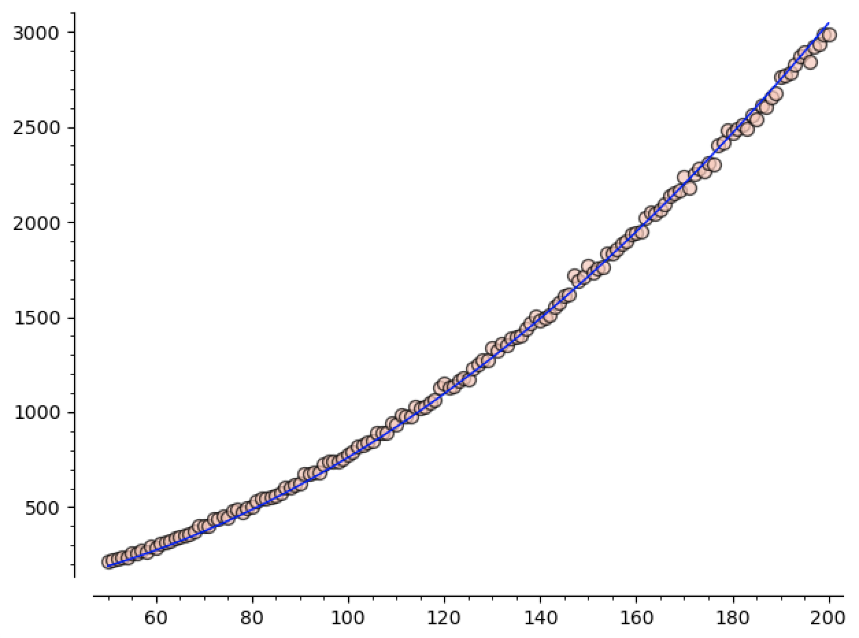
Since $1 / 16 = 0.0625$ , we see that, at least in the sizes we’re sampling, roughly $80 %$ of our regions are singletons.

We can check how good this model is, both inside and outside the range of data we used to define it, by running a few more tests.

For instance, running $getNumCCs (100, 50)$ will run another 50 tests on graphs of size $100 \times 100$ , then return the average number of regions over these tests. Simply plugging in gives us $guess (100) = 761.1$ , and running $getNumCCs (100, 50)$ gives an average of $772.76$ regions.

That’s pretty good! But how well does $guess$ predict the number of regions for $n$ outside the range of data we initially used?

$guess (300) = 6850$ , and empirically we find $getNumCCs (300, 50) = 6785.98$ !
Let’s push our luck! Sage tells us $guess (500) = 19027$ , and empirically $getNumCCs (500, 50) = 18343.5$

I’m definitely calling these a “win” for the formula!

They’re drifting apart, and I’m sure that’s because the model isn’t completely right. The standard deviation for how many regions we get is also growing as a function of $n$ , so we might also need more than $50$ samples in this range to get closer to the true average? I’m not a statistician, haha².

Regardless, this brings me to the first $\sim ⋆ \sim Conjecture \sim ⋆ \sim$ of the post!

Conjecture:

(Easy?): The expected number of regions in an $n \times n$ graph is $< 0.1 n^{2}$
(Hard?): Pin down the constant in the expected number of regions $C n^{2}$

Again, I’m not a probabilistic combinatorialist, so these sorts of questions are a bit outside my wheelhouse. I can’t tell if they’re either quite simple or almost impossible, but I know I (unfortunately) have other things to work on³ and can’t spend any more time on this. Hopefully one of you will be able to tackle these! ^_^

Lastly, the maximum region size.

Let’s say we know that there are $\approx C n^{2}$ many regions. Then since we have $n^{2}$ cells to allocate among the regions, the average region should contain $1 / C$ many cells. So there must be a region which contains $\geq 1 / C$ cells.

Assuming the easy conjecture from the previous section ( $C < 0.1$ ), we see that there must be a region containing more than $10$ cells.

This is better than nothing, but the size of the largest reason seems to be growing with $n$ (see the graphs later on in this section), so having a constant lower bound is less than ideal.

We can do a bit better, though. We know that most of these regions are singletons! So the other regions are going to have to be bigger to compensate.

As a (fun?) exercise, can you lower bound the size of the largest region using this idea?

I’ll leave my attempt in a foothote⁴

Since I don’t have any more ideas for trying to solve this problem, let’s at least get some data and make a conjecture!

xxxxxxxxxx
 
def getMaxCCs(n, N, p=None, q=None):
  """
  get the mean and std dev size of the largest CC
​
  run @N many tests on graphs of size @n
  """
​
  maxCCs = []
  for k in range(N):
    print("Running test ", k, "/", N)
    ccSizes = runTest(n,p,q)
    maxCCs += [ccSizes[0]]
​
  return (mean(maxCCs), sqrt(variance(maxCCs)))
​
def runMaxCCTest(n0,n1,N,p=None,q=None):
  out = []
  for n in range(n0,n1+1):
    (m,s) = getMaxCCs(n,N,p,q)
    out += [(n,m.n())]
​
  return out
​
# maxCCData = runMaxCCTest(50,200,50)

If we plot this data, we can see how the size of the largest region is growing with $n$ :

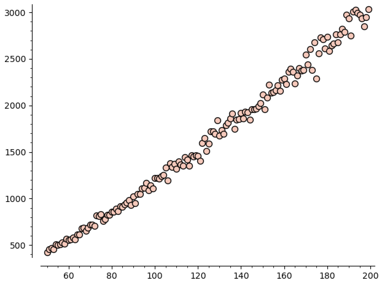
This plot really embarrasses the lower bound of $10$ that we got :P. You can read off the graph that it’s growing faster than linear, but how fast is it growing? Well, we can ask sage for a good polynomial model:

xxxxxxxxxx
 
a = var('a')
  b = var('b')
  model(n) = a * n^b
​
  sol = find_fit(maxCCData, model)
​
  guess(n) = model(a=sol[0].rhs(), b=sol[1].rhs())
​
  # this makes guess(n) = 1.9573061548255626*n^1.3888112924129952

Now we see the guess is

guess (n) \approx 1.95 n^{1.38} .

Plotting this against our data gives

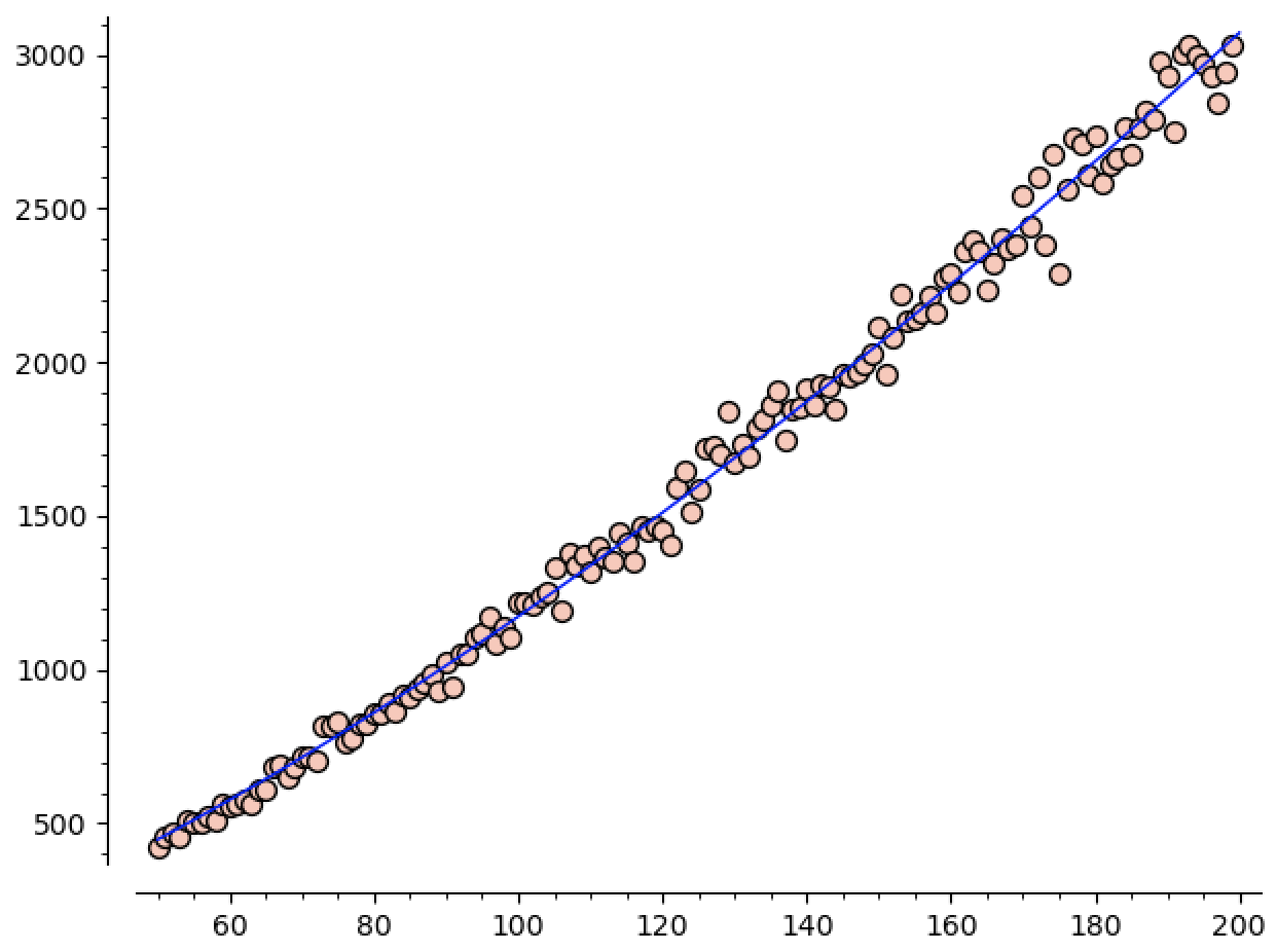
You can tell the standard deviation is higher here. Especially as $n$ increases. That said, we can still check the predictive value of our model.

$getMaxCCs (100, 50) = 1204.6$ , which lines up quite nicely with $guess (100) = 1172.9$ . In fact, they’re well within the standard deviation of $329$ (as computed by $getMaxCCs$ )
$getMaxCCs (300, 50) = 5163.2$ , which is still quite well approximated by $guess (300) = 5394$ . Indeed, the standard deviation is on the order of $1300$ , so our guess is doing quite well!
If we push our luck again and look at $getMaxCCs (500, 50) = 10617.2$ , our guess is $10965.2$ , which is still a good approximation! The standard deviation is $2952$ , so our model is killing it.
How far can we push things? If we run $getMaxCCs (1000, 50)$ , we get $27651.7$ , which somehow STILL matches up nicely with $guess (1000) = 28713.9$ . Especially seeing as the standard deviation is now almost $6000$ .

This data then leads to a new series of conjectures

Conjecture:

(Easy?) Can we show the expected size of the biggest region is $o (n^{2})$ ?
(Medium?) What about $o (n^{1.5})$ ?
(Hard?) Can we show that it is $Θ (n^{1.38})$ or so? What’s the exact exponent?
(Extremely Hard?) What’s the coefficient in front? We expect it’s probably $1.95 n^{1.38}$ or so, but… Can we know for sure?

I think this kind of use case for sage is really powerful! It’s a great tool not only for solving concrete problems that arise in research, but also for formulating new conjectures and playing around with lots of concrete examples at once! Hopefully this showcases another angle on how we can use sage in the wild to work on our research problems.

Also, again, if anyone makes any progress on these, please let me know! I would love to know anything you’re able to figure out ^_^

A huge thanks to Brandon Curtis for the blog of sage resources! In particular the model fitting example here was super helpful. ↩
Thankfully one of my best friends is a statistician. He’s been a huge help for this whole process, and you can find him on twitch ↩
I really want to start writing music so that I’ll have something by the end of the year. Also there’s the upcoming posts on fourier analysis, etc. ↩
We know that there are $\approx (1 / 16) n^{2}$ singleton regions. That means we have $\approx (C - (1 / 16)) n^{2}$ nonsingleton regions, and $(15 / 16) n^{2}$ remaining cells to distribute amongst these regions.

So the average nonsingleton region has $\frac{15 / 16}{C - (1 / 16)}$ cells, so there must be a particular region with at least that many cells.

Assuming the conjecture $C < 0.1$ , we see the largest region must have at least $25$ cells. This is better. But still independent of $n$ .

I don’t think this approach can be saved, either. We know the expected number of singletons, so the numerator can only be $15 / 16$ . Even if we guess there are error terms in the number of regions total, that gives us lower order terms in the denominator that go to $0$ as $n \to \infty$ …

We could also try including more small regions, say by counting plus signs as well as singletons. But this would just improve the constant (do you see why?). What we would need to know is that there’s a lot of “small” regions where “small” now isn’t a constant, but depends on $n$ . For instance, can we estimate the number of regions of size $\leq n$ ? ↩