A Follow Up -- Explicit Error Bounds

05 Jan 2022 - Tags: quick-analysis-tricks , sage

In my previous post I talked about how we can use probability theory to make certain scary looking limits obvious. I mentioned that I would be writing a follow up post actually doing one of the derivations formally, and for once in my life I’m going to get to it quickly! Since I still consider myself a bit of a computer scientist, it’s important to know the rate at which limits converge, and so we’ll keep track of our error bounds throughout the computation. Let’s get to it!

Let $f : R \to R$ be bounded and locally lipschitz. Then for every $x > 0$ ,

$e^{- n x} \sum_{k = 0}^{\infty} \frac{(n x)^{k}}{k!} f (\frac{k}{n}) = f (x) \pm {\tilde{O}}_{x} (\frac{1}{\sqrt{n}})$

$⌜$

In the interest of exposition, I’ll show far more detail than I think is required for the problem. Hopefully this shows how you might come up with each step yourself.

Let $X_{n}$ be poisson with parameter $n x$ . Then notice

e^{- n x} \sum_{k = 0}^{\infty} \frac{(n x)^{k}}{k!} f (\frac{k}{n}) = E [f (\frac{X_{n}}{n})]

Now we compute

\begin{aligned} | E [f (\frac{X_{n}}{n})] - f x | & = | \int f (\frac{X_{n}}{n}) d P (X_{n}) - \int f x d P (X_{n}) | \\ = | \int f (\frac{X_{n}}{n}) - f x d P (X_{n}) | \end{aligned}

Now we use an extremely useful trick in measure theory! We’ll break up this integral into two parts. One part where the integrand behaves well, and one part (of small measure) where the integrand behaves badly.

Using our intuition that $\frac{X_{n}}{n} \approx x$ , we’ll partition into two parts:

$| \frac{X_{n}}{n} - x | < δ_{n}$ (the “good” set)
$| \frac{X_{n}}{n} - x | \geq δ_{n}$ (the “bad” set)

We’ll be able to control the first part since there our integrand is $\approx 0$ , and we’ll be able to control the second part since it doesn’t happen often. Precisely, we’ll use a chernoff bound. There’s a whole zoo of things called “chernoff bounds”, all subtly different, but any one of them will be good enough for our purposes here. I’m just using the first one that came up when I googled “poisson chernoff bounds” :P.

So we split our integral:

\begin{aligned} | \int f (\frac{X_{n}}{n}) - f x d P (X_{n}) | \\ \leq | \int_{| \frac{X_{n}}{n} - x | < δ_{n}} f (\frac{X_{n}}{n}) - f x d P (X_{n}) | + | \int_{| \frac{X_{n}}{n} - x | \geq δ_{n}} f (\frac{X_{n}}{n}) - f x d P (X_{n}) | \\ \leq \int_{| \frac{X_{n}}{n} - x | < δ_{n}} | f (\frac{X_{n}}{n}) - f x | d P (X_{n}) + \int_{| \frac{X_{n}}{n} - x | \geq δ_{n}} | f (\frac{X_{n}}{n}) - f x | d P (X_{n}) \end{aligned}

Now since $f$ is locally lipschitz, we know that in a neighborhood of $x$ , we must have $| f (y) - f (x) | \leq M_{x} | y - x |$ . So for $δ_{n}$ small enough, we’ll have (in the “good” set)

| f (\frac{X_{n}}{n}) - f x | \leq M_{x} | \frac{X_{n}}{n} - x | \leq M_{x} δ_{n}

Since $f$ is bounded, say by $‖ f ‖_{\infty}$ , we know that no matter what we’ll have

| f (\frac{X_{n}}{n}) - f x | \leq | f (\frac{X_{n}}{n}) | + | f x | \leq 2 ‖ f ‖_{\infty}

Putting these estimates into the above integral, we find¹

\begin{aligned} \leq \int_{| \frac{X_{n}}{n} - x | < δ_{n}} M_{x} δ_{n} d P + \int_{| \frac{X_{n}}{n} - x | \geq δ_{n}} 2 ‖ f ‖_{\infty} d P \\ = (M_{x} δ_{n}) P (| \frac{X_{n}}{n} - x | \geq δ_{n}) + 2 ‖ f ‖_{\infty} P (| \frac{X_{n}}{n} - x | \geq δ_{n}) \end{aligned}

since we can pull the constants out of the integral, then get the measures of the “good” and “bad” sets.

Now the good set has measure at most $1$ ², and chernoff bounds show that the bad set has exponentially small measure:

\begin{aligned} P (| \frac{X_{n}}{n} - x | \geq δ_{n}) & = P (| X_{n} - n x | \geq n δ_{n}) \\ \leq 2 \exp (\frac{- (n δ_{n})^{2}}{2 (x n + n δ_{n})}) \\ = 2 \exp (\frac{- n δ_{n}^{2}}{2 (x + δ_{n})}) \end{aligned}

So plugging back into our integral, we get

\leq M_{x} δ_{n} + 2 ‖ f ‖_{\infty} 2 \exp (\frac{- n δ_{n}^{2}}{2 (x + δ_{n})})

We want to show that this goes to $0$ , and all we have is control over the sequence $δ_{n}$ . $M_{x}$ is a constant, so we have to have $δ_{n} \to 0$ . Likewise $4 ‖ f ‖_{\infty}$ is a constant, so we need $\exp (\frac{- n δ_{n}^{2}}{2 (x + δ_{n})}) \to 0$ . Since the stuff in the exponent is negative and $2 (x + δ_{n}) \approx 2 x$ is a constant, that roughly means we need $n δ_{n}^{2} \to \infty$ .

We can choose any $δ_{n}$ we like which satisfies these two properties, but it’s somewhat difficult to find something that works. We notice that $δ_{n} = n^{- \frac{1}{2}}$ just barely fails, since $n^{- \frac{1}{2}} \to 0$ , but $n {(n^{- \frac{1}{2}})}^{2} \to 1$ .

If we pick $δ_{n}$ just a smidge bigger than $n^{- \frac{1}{2}}$ , say, $n^{- \frac{1}{2}} \log (n)$ , that should get the job done³. Clearly $M_{x} n^{- \frac{1}{2}} \log (n) = \tilde{O} (n^{- \frac{1}{2}})$ , and moreover

\exp (\frac{- n {(n^{- \frac{1}{2}} \log (n))}^{2}}{2 (x + n^{- \frac{1}{2}} \log (n))}) = n^{- \frac{1}{2} \frac{1}{\frac{x}{\log (n)} + \frac{1}{\sqrt{n}}}}

and a tedious L’hospital rule computation shows that this is eventually less than $n^{- \frac{1}{2}} \log (n)$ .

So what have we done?

We started with

| e^{- n x} \sum_{k = 0}^{\infty} \frac{(n x)^{k}}{k!} f (\frac{k}{n}) - f (x) | = | E [f (\frac{X_{n}}{n})] - f (x) |

and we showed this is at most

M_{x} δ_{n} + 2 ‖ f ‖_{\infty} 2 \exp (\frac{- n δ_{n}^{2}}{2 (x + δ_{n})}) = O_{x} (\frac{\log (n)}{\sqrt{n}}) = {\tilde{O}}_{x} (\frac{1}{\sqrt{n}})

So, overall, we have

e^{- n x} \sum_{k = 0}^{\infty} \frac{(n x)^{k}}{k!} f (\frac{k}{n}) = f (x) \pm {\tilde{O}}_{x} (\frac{1}{\sqrt{n}})

as promised.

$⌟$

After I got through with this proof, I wanted to see if it agreed with some simple experiments. The last step of this, where we played around with the $δ_{n}$ s, was really difficult for me, and if your math is making a prediction, it’s a nice sanity check to go ahead and test it.

So then, let’s try to approximate some functions! I’ve precomputed these examples, but you can play around with the code at the bottom if you want to.

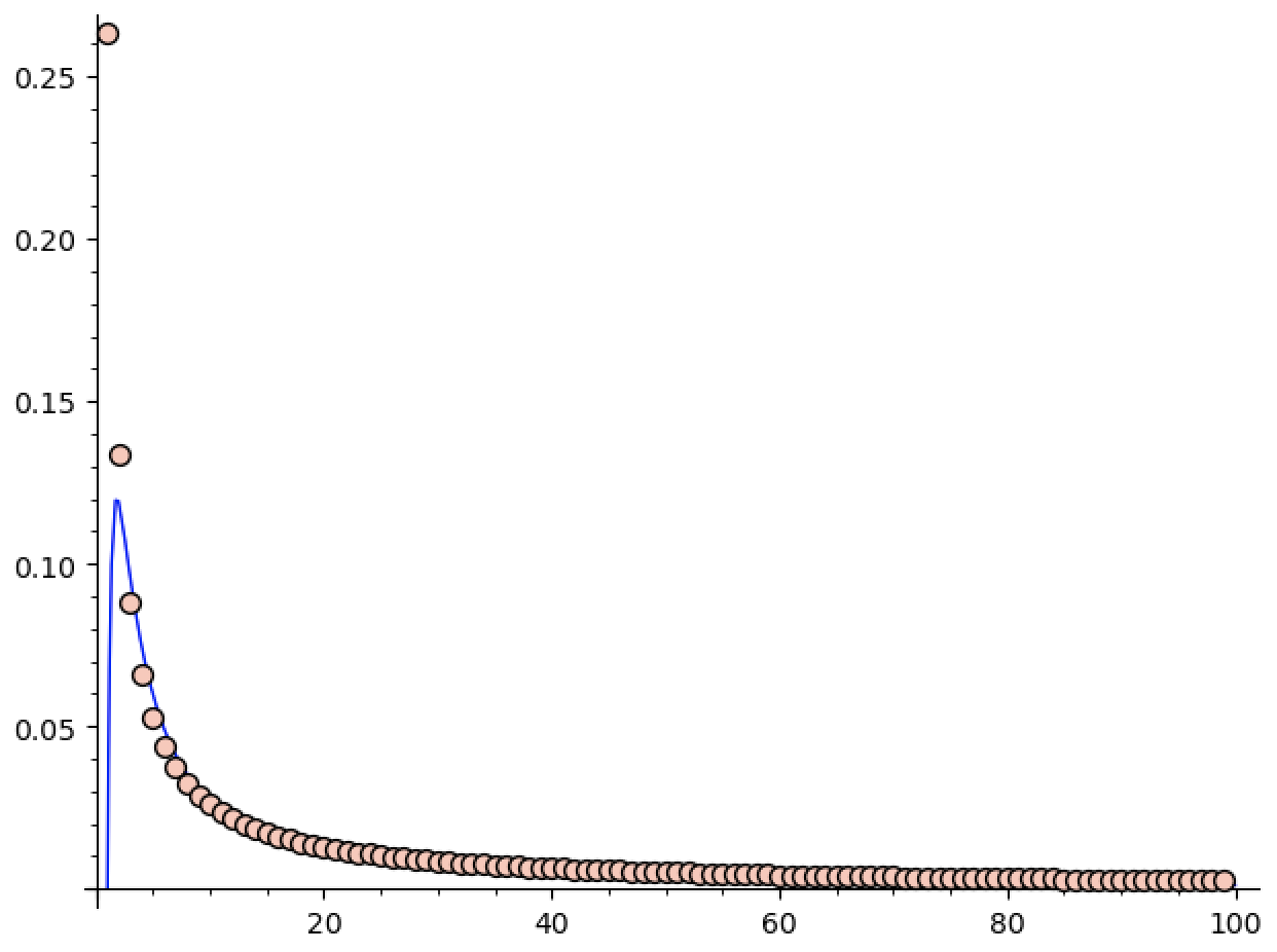
First, let’s try to approximate $\sin (3 / 4)$ using this method. We get nice decay, but it’s much faster than $\frac{\log (n)}{\sqrt{n}}$ . Indeed, sage guesses it’s closer to $\frac{\log (n)}{n^{1.6}}$ .

(Edit: I realized I never said what these pictures represent. The $x$ axis is the number of terms used, and the $y$ axis is the absolute error in the approximation. You can figure this out based on the code below, but you shouldn’t need to understand the code to understand the graphs so I’m adding this little update ^_^.)

That’s fine, though. It’s more than possible that I was sloppy in this derivation, or that tighter error bounds are possible (especially because $\sin$ is much better behaved than your average bounded locally lipschitz function).

So let’s try it on a more difficult function⁴. What if we try to approximate $\sin (1 / (0.001 + x))$ at $x = 0.1$ . (We have to perturb things a little bit so the code doesn’t divide by $0$ anywhere).

Now we get some oscillatory behavior, which seems to be stabilizing.

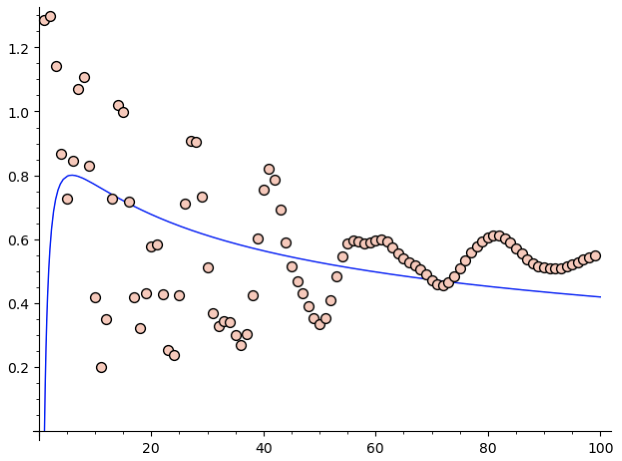
At least the guess in this case is closer to what we computed, as the blue graph is roughly $1.23 \frac{\log n}{n^{0.56}}$ . This obviously isn’t an upper bound for our data, but it’s only off by a translation upwards, and they do seem to be decaying at roughly the same rate.

The fact that this example gives something fairly close to the bounds we ended up getting makes me feel better about things. In fact, after a bit of playing around, I can’t find anything where sage guesses the decay is slower than $\frac{\log (n)}{\sqrt{n}}$ , which also bodes well.

If you want to play around for yourself, I’ve left the sage code below!

xxxxxxxxxx
 
def approx(f,x,n, verbose=False):
  """
  Compute the nth approximation of f at x according to our formula
  """
  total = 0
​
  # We're only summing the first 500 terms of the series,
  # and that causes some distortion for large values of n
  for k in range(500): 
    total += (exp(-n*x) * ((n*x)^k / factorial(k)) * f(x=k/n)).n()
​
  return total.n()
​
​
def test(f, N=100, x=None, showPlot=False):
  """
  Get the error between f(x) and approx(f,x,n) as n goes from 1 to @N.
​
  If no x is given, pick one randomly in (-1,1).
​
  Return the error data, and plot it if @showPlot is true
  """
​
  if x == None:
    x = RR(uniform(-1,1))
​
  target = f(x=x).n()
​
  data = []
​
  n = 1
  while n < N:
    a = approx(f,x,n)
    data += [ (n, abs(a - target)) ]
​
    n += 1
​
  a,b,n = var('a,b,n')
  model(n) = a * n^b * log(n)
  sol = find_fit(data,model)
  guess(n) = model(a=sol[0].rhs(), b=sol[1].rhs())
​
  show(guess)
​
  if showPlot:
    scatterPlot = scatter_plot(data)
    guessPlot = plot(guess, n, 1, N)
​
    show(scatterPlot + guessPlot)
​
  return (x, guess, data)
​
@interact
def _(f=sin(x), x=3/4, auto_update=False):
  _ = test(f, x=x, showPlot=True)

Help | Powered by SageMath

Accepted: {"data":{"application/sage-clear":{"changed":["f","x","auto_update"]},"text/plain":"Clear display"},"source":"sagecell"}

Accepted: {"data":{"application/sage-interact":{"new_interact_id":"a2ccf5df-e9b7-492a-b85d-7f167a918d65","controls":{"f":{"control_type":"input_box","subtype":"input","default":"sin(x)","width":0,"height":1,"evaluate":true,"keypress":false,"label":"f","update":false},"x":{"control_type":"input_box","subtype":"input","default":"3/4","width":0,"height":1,"evaluate":true,"keypress":false,"label":"x","update":false},"auto_update":{"control_type":"button","width":"","text":"Update","raw":true,"label":"","update":true}},"layout":[[["f",1]],[["x",1]],[["auto_update",1]],[["_output",1]]],"locations":null,"readonly":false},"text/plain":"Sage Interact"},"source":"sagecell"}

Messages

I’m pretty confident in what we’ve done today, but I can’t help but feel like there’s a better way, or that there’s slightly tighter bounds to be had. If there’s anyone particularly skilled in “hard” analysis reading this, I would love to hear your thoughts ^_^.

In any case, this has been fun to work through! I’ll see you all soon!

In the interest of continuing the quick analysis trick tradition of saying the obvious thing, notice what we’ve done here. We want to control an integral. How do we do it?

We break it up into a “good” piece, which is big, and a “bad” piece, which is small.

The “good” piece we can control because it’s good. For us, this means $f (\frac{X_{n}}{n}) \approx f (x)$ , so their difference is $\approx 0$ .

The “bad” piece we can’t control in this way. Indeed it’s defined to be the piece that we can’t control in this way. Thankfully, if all is right with the world, the “bad” piece will be small! So we get some crummy (uniform) estimate on the bad piece, and then multiply by the size of the piece. Since the size is going to $0$ and our bound is uniform (even if it’s bad), we’ll win! ↩
Notice just like we were content with a crummy bound on the integrand of the bad piece because we’re controlling the measure, we’re content with a potentially crummy bound on the measure of the good piece because we’re controlling the integrand!

Of course, for our particular case, $1$ is actually a fairly good bound for the measure of the good piece, but we don’t need it to be. ↩
In fact, $δ_{n} = n^{- \frac{1}{2} + ϵ}$ also gets the job done, but the computation showing
$\exp (\frac{- n δ_{n}^{2}}{2 (x + δ_{n})}) = O (δ_{n})$
is horrendous. ↩
Interestingly, while trying to break things, I realized that I don’t really have a good understanding of “pathological” bounded lipschitz functions. Really the only tool in my belt is to make things highly oscillatory…

Obviously we won’t have anything too pathological. After all, every (globally) lipschitz function is differentiable almost everywhere, and boundedness means we can’t just throw singularities around to cause havoc. But is oscillation really the only pathology left? It feels like there should be grosser things around, but it might be that they’re just hard to write down.

Again, if you have any ideas about this, I would also love to hear about it! ↩