Finiteness in Sheaf Topoi

19 Aug 2024 - Tags: topos-theory

The notion of “finiteness” is constructively subtle in ways that can be tricky for people new to the subject to understand. For a while now I’ve wanted to figure out what’s going on with the different versions of “finite” in a way that felt concrete and obvious (I mentioned this in a few older blog posts here and here), and for me that means I want to understand them inside a sheaf topos $\mathsf{Sh}(X)$. I’ve thought about this a few times, but I wasn’t able to really see what was happening until a few days ago when I realized I had a serious misconception about picturing bundles and etale spaces! In this post, we’ll talk about that misconception, and spend some time discussing constructive finiteness in its most important forms.

As a short life update before we get started, I’m currently in Denmark with my advisor to hang out with Fabian Haiden. We’re going to be talking about all sorts of fun things related to my thesis work, mainly about Fukaya Categories. These can be really scary when you first start reading about them, but in the special case of surfaces they’re really not that bad! In the process of prepping for meeting Fabian, I’ve been writing a blog post that explicitly details what fukaya categories are, why you should care, and (for surfaces) how to compute them. I know I would have loved an article like this, and I’m excited to share one soon! I’m also finally going to finish my qual prep series from three years ago! Way back then I promised a post on fourier theory that I never got around to, but I recently found a draft of that post! So it might not be 100% true to what I was studying back then, but it’ll be as true to that as I can make it¹.

With all that out of the way, let’s get to it!

---

First, let’s just recall the notions of finiteness you’re likely to find in the literature². Keep in mind that, depending on the reference you’re reading, each of these is liable to be called just “finite” without disambiguation. Sometimes you even get more confusing conventions, (such as writing “subfinite” to mean what we call “kuratowski finite”!) so make sure you read carefully to know exactly what each particular author means! For this post, though, we’ll write:

If $n : \mathbb{N}$, the Finite Cardinal of size $n$ is the set \([n] = \{ x : \mathbb{N} \mid x \lt n \}\).

A set $X$ is called Bishop Finite if it’s (locally) isomorphic to a cardinal. That is, if \(\exists n : \mathbb{N} . \exists f : X \cong [n]\)

A set $X$ is called Kuratowski Finite if it’s (locally) the image of a cardinal. That is, if \(\exists n : \mathbb{N} . \exists f : [n] \twoheadrightarrow X\).

A set $X$ is called Subfinite if it’s (locally) a subobject of a cardinal. That is, if \(\exists n : \mathbb{N} . \exists f : X \hookrightarrow [n]\).

A set $X$ is called Dedekind Finite if every mono $X \hookrightarrow X$ is actually an iso. That is, if we can prove \(\forall f : X \hookrightarrow X . \exists g : X \to X . fg = 1_X \land gf = 1_X\).

It’s pretty obvious from these definitions that dedekind finiteness is a bit different from the others. This comes with pros and cons, but in my experience it’s rarely the thing to consider. I’m including its definition more for cultural growth than anything, and I won’t say anything more about it in this post³.

Also, notice we’re putting an existential quantifier in front of everything. Externally, this means that we’re allowed to pass to an open cover of our base space and use a different $f$ (or indeed, a different $n$!) on each open. If you prefer type theory⁴, you can replace every instance of $\exists$ by the propositional truncation of a $\Sigma$-type.

It’s interesting to ask what the “untruncated” versions of these will be. I think that untruncated bishop finite types are exactly the cardinals, untruncated subfinite types are disjoint unions of finitely many propositions… But it’s not clear to me what the untruncated kuratowski finite types should be. Something like “finitely many copies of $B$, glued together along open sets”… But I don’t see a snappy characterization of these⁵.

---

Introducing Finiteness

Now, how should we go about visualizing these things? Every sheaf on $B$ is also an etale space over $B$ (that is, a local homeomorphism⁶ $E \to B$). And by thinking of our favorite sheaf as some space over $B$ we can draw pictures of it!

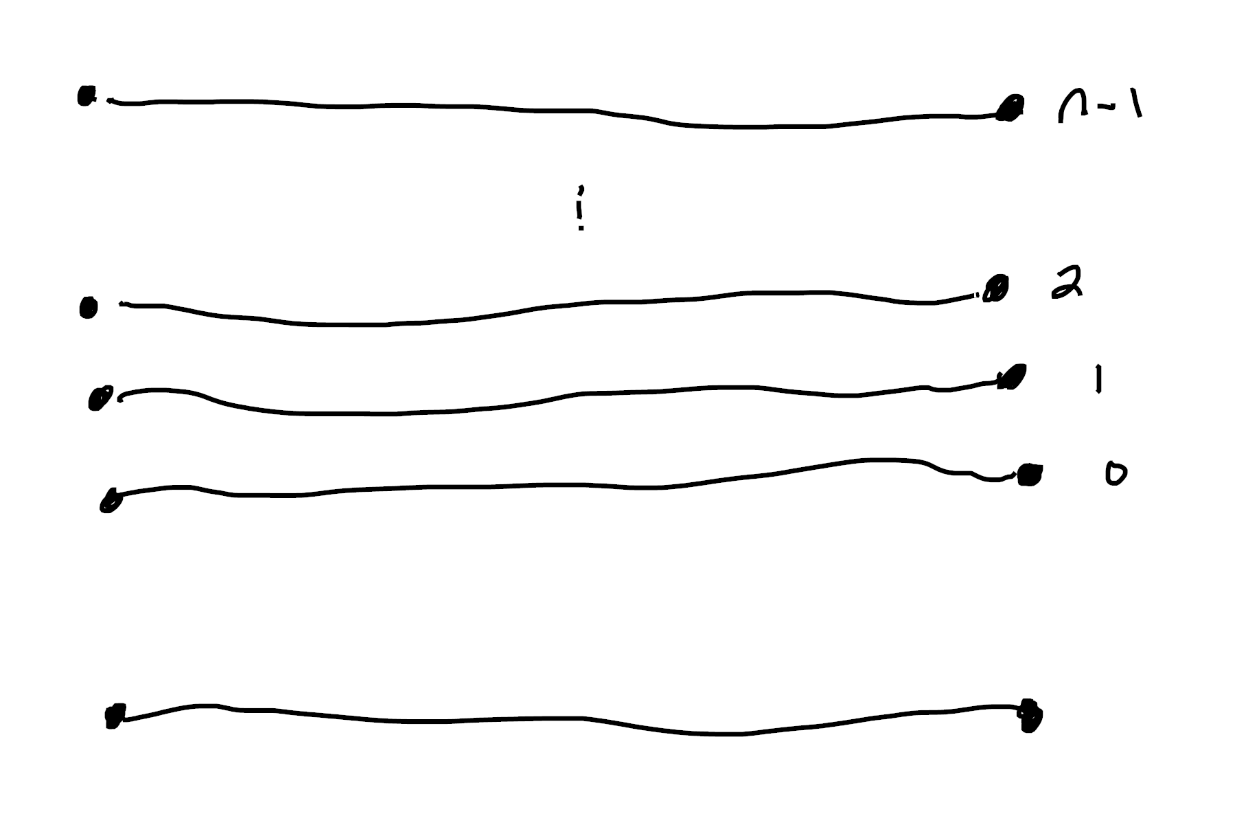
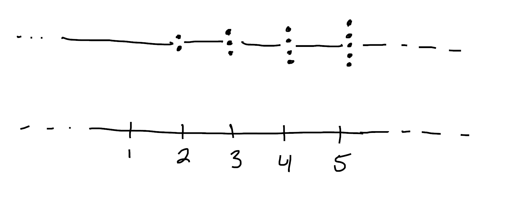
Let’s start simple and let $B = [-1,1]$ be an interval. Then a cardinal⁷ is a sheaf \([n] = \{x : \mathbb{N} \mid x \lt n \}\). In every sheaf topos $\mathsf{Sh}(B)$ the natural number object is (the sheaf of sections of) $B \times \mathbb{N}$ where $\mathbb{N}$ gets the discrete topology.

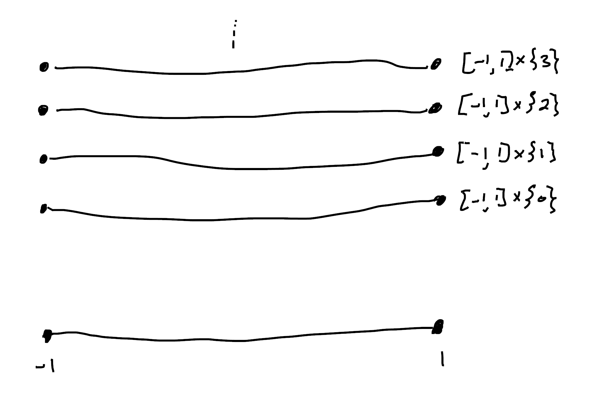
So if $n$ is a global section, it must be \(B \times \{ n \}\) for some fixed $n$ in “the real world”. This also tells us that \([n] = \{ x : \mathbb{N} \mid x \lt n \}\) is given by

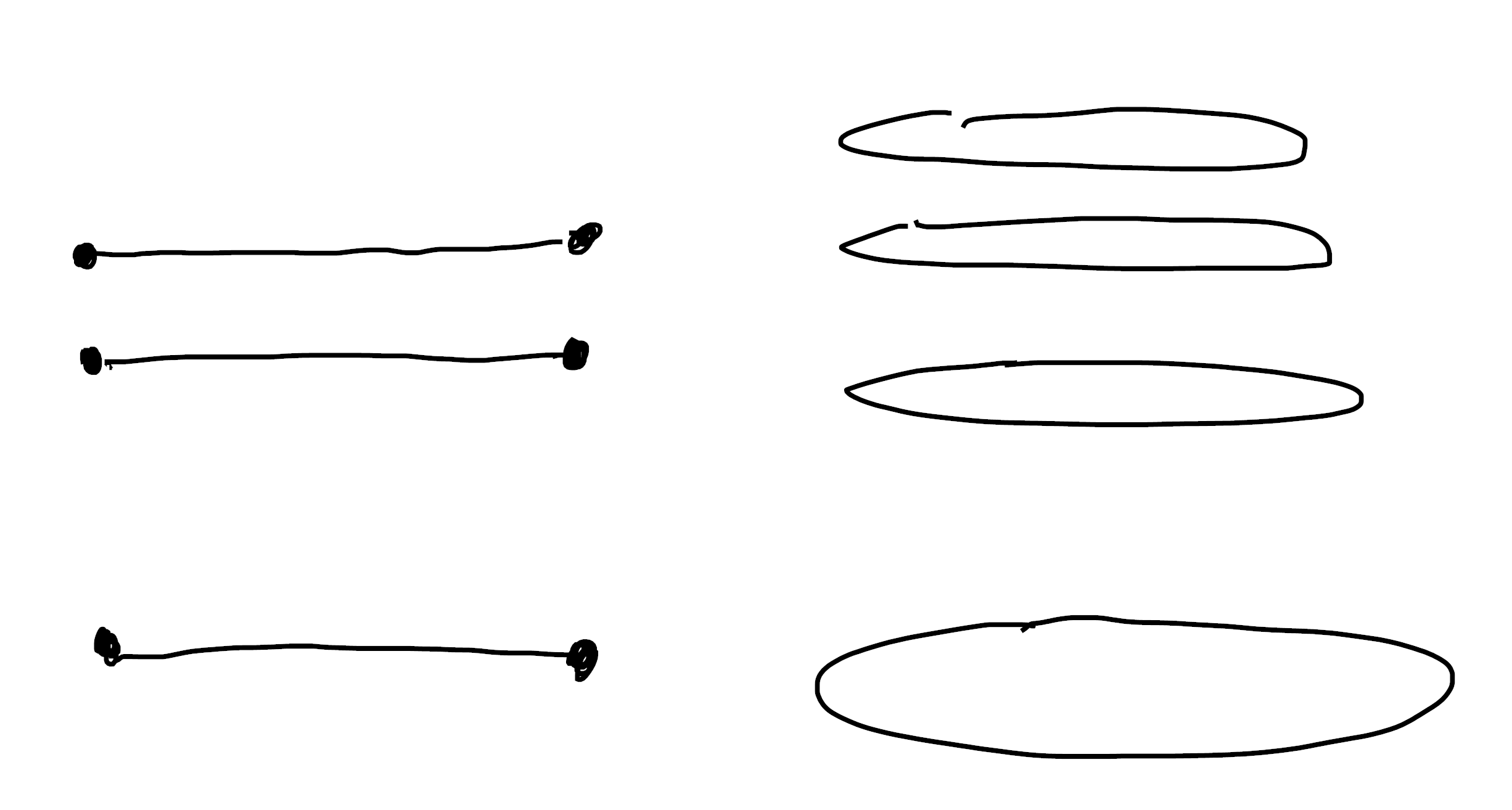
The situation is only slightly more complicated if $B$ has multiple components⁸ (say $B = [-1,1] \sqcup S^1$). In this case, $\mathbb{N}$ is still $B \times \mathbb{N}$, but now global sections can choose a different natural over each component:

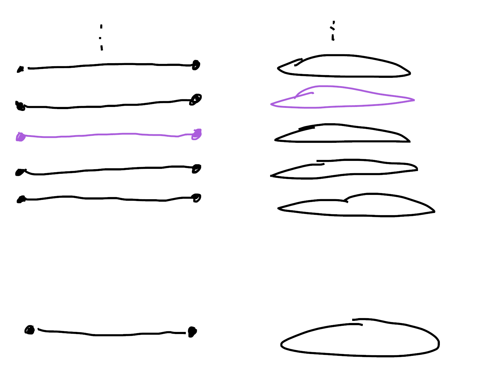
Because of this, we end up with more sets $[n]$! Indeed, now a global section $n$ might be something like $(2,3)$ (shown in pink above) so that we get a cardinal $[(2,3)]$, shown below:

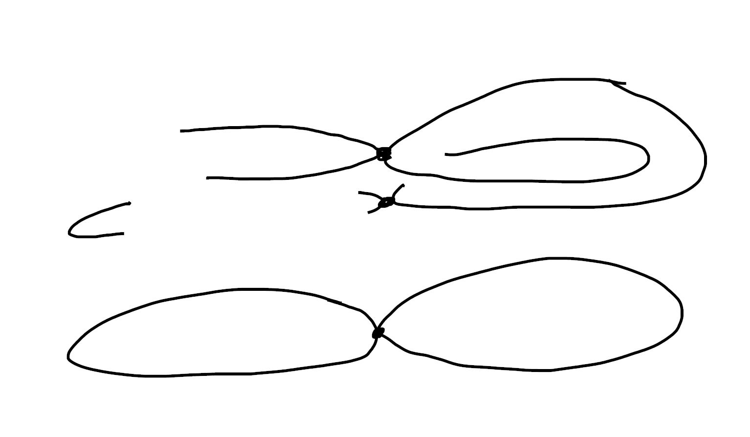
So cardinals are really really easy to work with! This is what we would expect, since they’re subsheaves of a particularly simple sheaf ($\mathbb{N}$). For instance, we can see the fact that cardinals always have decidable equality by noticing that any two sections over $U$ are either equal on all of $U$, or none of $U$! Contrast this with a doodle of what other sheaves might look like, where the pink and blue sections are different, but nonetheless intersect. Then the truth value of $(\text{pink} = \text{blue}) \lor (\text{pink} \neq \text{blue})$ as computed in $\mathsf{Sh}([-1,1]) \big / U$ will not be all of $U$⁹!

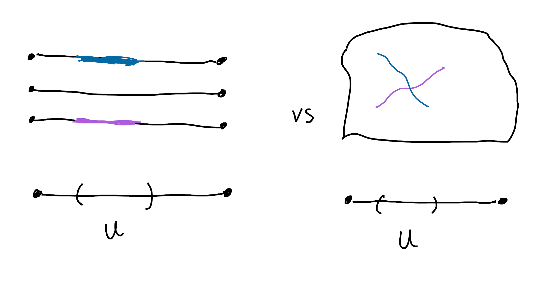
We also see why a cardinal is either empty or inhabited! As soon as you have a piece of a section over $U$, it must extend to a section on all of $U$.

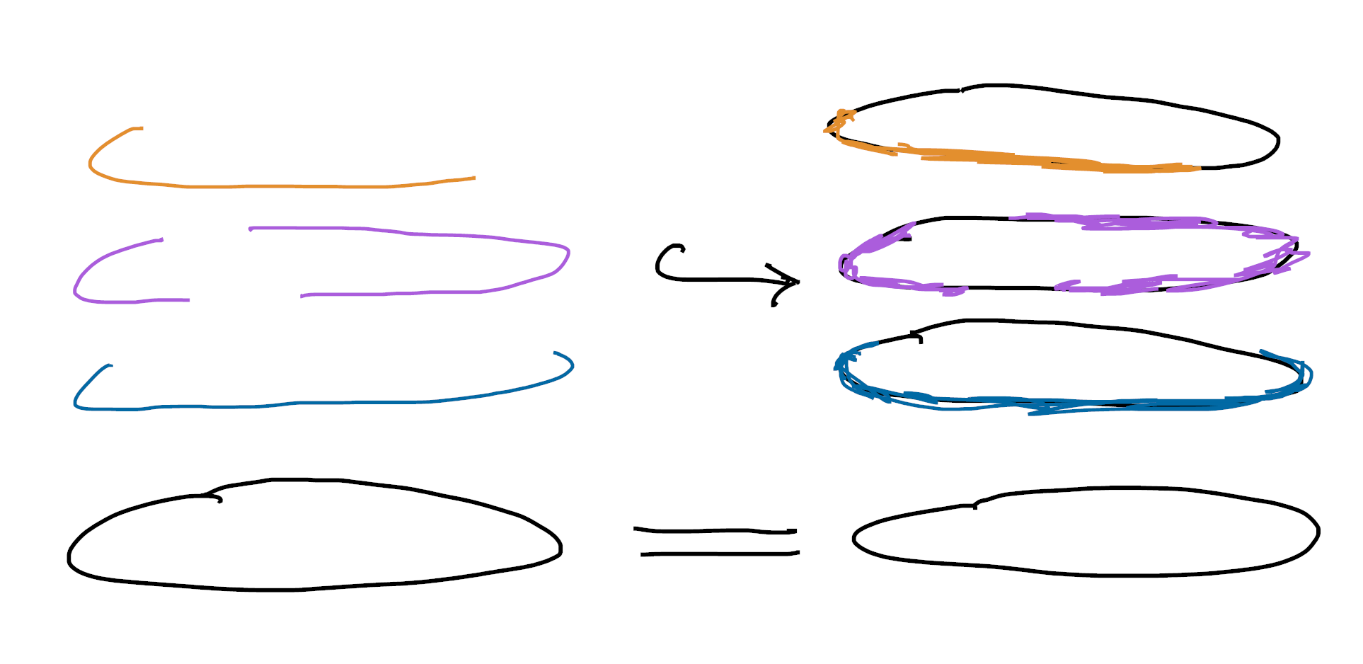
Next up are the bishop finite sets¹⁰! These satisfy $\exists f : X \cong [n]$, so that we can find an open cover \(\{U_\alpha \}\) of $B$ and functions \(f_\alpha : X \! \upharpoonright_\alpha \cong [n] \! \upharpoonright_\alpha\).

Since $[n]$ is a constant family over $B$, this means we want $X$ to be locally constant. So bishop finite sets have to basically look like cardinals, but now we’re allowed to “twist” the fibres around. See how on each element of our cover we have something that looks like $[2]$, but globally we get something that is not isomorphic to $[2]$!

In fact, the bishop finite sets are exactly the covering spaces with finite fibres. These inherit lots of nice properties from the cardinals, since as far as the internal logic is concerned they’re isomorphic to cardinals!

For instance, here’s an internal proof that bishop finite sets have decidable equality:

$\ulcorner$ We know $\exists f : X \cong [n]$. Fix such an $f$, and let $x,y : X$. Since $f$ is an isomorphism we know $x=y$ if and only if $fx = fy$, but we can decide this using decidable equality on $[n]$ (which comes from decidable equality on $\mathbb{N}$, which we prove by induction). $\lrcorner$

We can also see this externally. As before, this is saying that two sections over $U$ either agree everywhere or nowhere (and it’s a cute exercise to see this for yourself). But we can even see this in a third way! It says that the subsheaf \(\{(x,y) : X \times X \mid x=y \}\) is a clopen subset of $X \times X$! But we can compute $X \times X$ (the pullback of $X \to B$ along $X \to B$) and check this.

Note that the subsheaf (really sub-etale space) where the fibres are the same really is a clopen subset (read: a connected component) of the whole space $X \times X$ over $B$. If it’s not obvious that this really is the pullback, it makes a fun exercise! Actually, it’s a fun exercise to check this is true in general!

As a last remark, let’s also notice that bishop finite sets can be inhabited without being pointed. That is, a bishop finite set $X$ can satisfy $\exists x : X$ ($X$ is inhabited¹¹) without actually having $x:X$ for any $x$ ($X$ is not pointed)! This is because of the locality of the existential quantifier again! If we pass to an open cover of $B$, we can find a local section over each open. Unfortunately, these might not be compatible, so won’t glue to a global section (a point $x:X$)!

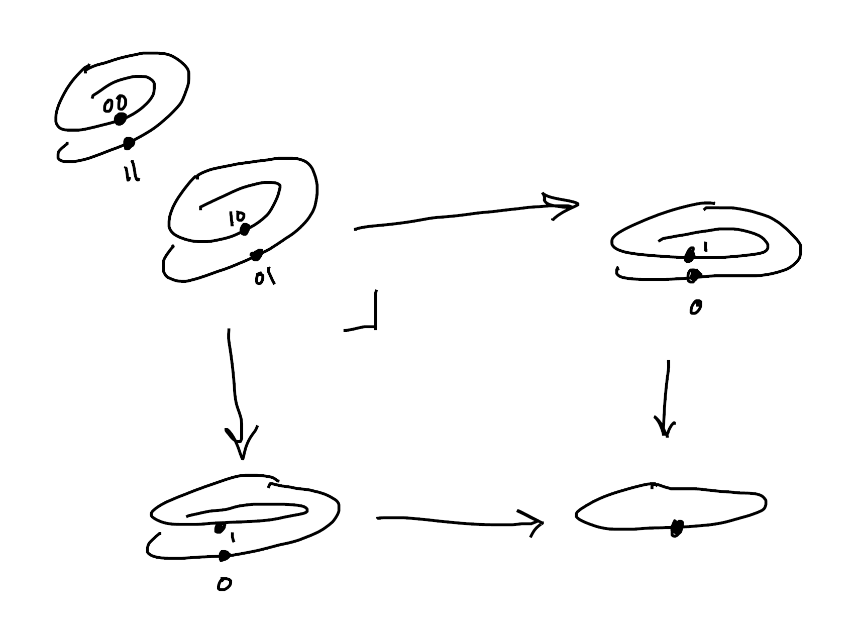
Ok, now let’s get to the example that led me to write this post! How should we visualize kuratowski finite sets? These are (locally) quotients of cardinals, so we start with a cardinal (which we know how to visualize) and then we want to start gluing stuff together.

Let’s start with a trivial double cover of $B = [-1,1]$ (that is, with two copies of $B$), and glue them together along their common open subset $[-1,0) \cup (0,1]$. This space is the line with two origins, and it’s famously nonhausdorff!

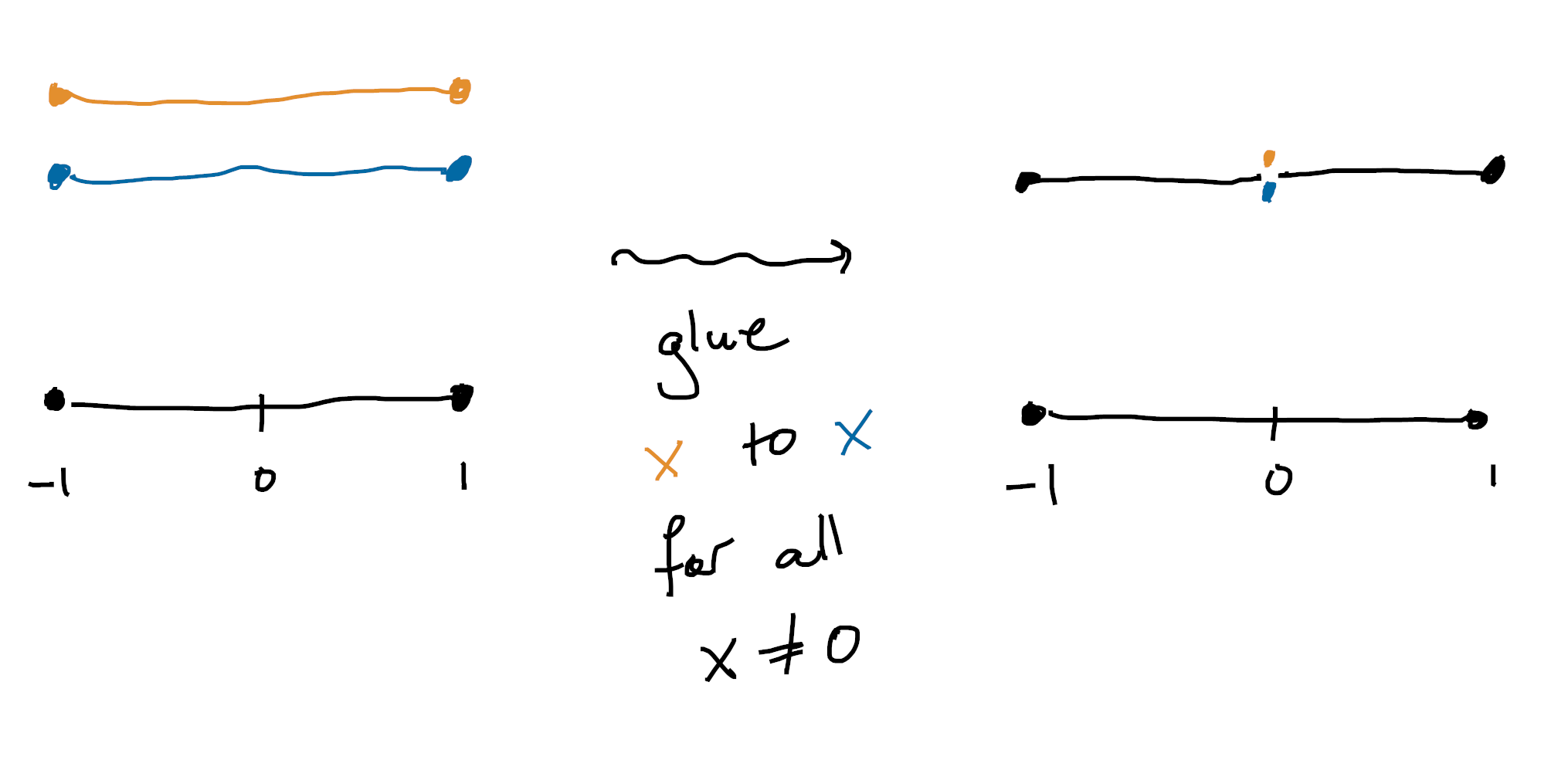
You can see that this space still deserves to be called “finite” over $B$ (for instance, all the fibres are finite), but it’s more complicated than the bishop case. For instance, it doesn’t have a well defined “cardinality”. In some places it has one element in the fibre, and in others it has two. However, it’s still possible to list or enumerate all the sections. In the above picture, there’s the gold section and the blue section. It just happens that sometimes this list has duplicates, since away from $0$ they’re the same section!

The failure of hausdorffness and the failure of decidable equality are closely related. For example, consider the two sections from the previous picture. Decidable equality says that they should be either everywhere equal or everywhere unequal¹². But of course they aren’t! They’re equal in some places (over $1$, say) but unequal in others (over $0$)!

Following Richard Borcherds, hausdorffness is also closely related to a kind of “analytic continuation”. Indeed, say your etale space $X$ is hausdorff and you pick a point $x_b$ over $b \in B$ (in this context we think of $x_b$ as the germ of a function at $b$). Then for any small enough open $U \ni b$, there is a unique extension of $x_b$ to a function on the whole neighborhood $U$! We are able to analytically continue $x_b$ from data at just a point to data defined in some neighborhood!

solution

$\ulcorner$

First assume $\mathcal{F}$ has a hausdorff etale space $X$. Then for sections $f,g : U \to X$ we see that the set $\{b \in U \mid f(b) = g(b) \}$ is closed, as the preimage of the closed diagonal in $X$. This set is also open since if $f(b) = g(b)$ is the stalk at $b$, the definition of stalk says that $f=g$ on a neighborhood of $b$. Since $U$ is connected, we learn this subset is the whole of $U$ and $\mathcal{F}$ has analytic continuation.

Conversely, assume $\mathcal{F}$ has analytic continuation, and let $x,y \in X$ be two points. If $x$ and $y$ are in different fibres (say $x$ is over $b_x$ and $y$ is over $b_y$) then we can separate $b_x$ and $b_y$ using hausdorfness of $B$, and any representatives of $x$ and $y$ defined on these separating sets will separate $x$ and $y$ in $X$. So we're left with the case of $x$ and $y$ both living in the same fibre over $b$.

Say that every neighborhood of $x$ intersects every neighborhood of $y$. Using local connectedness of $B$, we can find a connected neighborhood $U$ of $b$, and representatives $(f,U)$ and $(g,U)$ of $x$ and $y$. These define open sets in the topology of $X$, and since neighborhoods of $x$ and $y$ always intersect, we know there's a $b' \in U$ with $f(b') = g(b')$. Then analytic continuation says $f=g$ on $U$ so that $x = f(b) = g(b) = y$, and $X$ is hausdorff, as desired.

$\lrcorner$

When I was trying to picture kuratowski finite objects inside $\mathsf{Sh}(B)$, I’d somehow convinced myself that a local homeomorphism over a hausdorff space has to itself be hausdorff. This is, obviously, not true! So I was trying to picture kuratowski finite sets and struggling, because I was only ever picturing hausdorff covering spaces. And we’ll see later that all hausdorff kuratowski finite sheaves (over spaces I was picturing) are actually bishop finite! So it’s no wonder I was confused! I didn’t realize the complexity (especially the nonhausdorff complexity) that etale spaces are allowed to have, even though in hindsight I’d been warned about this before¹⁴.

Going back to examples, we should ask if we recognize the sheaf of sections for our favorite “line with two origins” picture from earlier. Away from $0$, we know there’s exactly one section, but in any neighbordhood of $0$ there’s two sections. So we see this is the etale space for the skyscraper sheaf with two points over $0$!

Since our epi $[n] \twoheadrightarrow X$ only has to exist locally, kuratowski finite objects in $\mathsf{Sh}(B)$ can have the same twisting behavior as bishop finite sets too!

If you look up an example of a kuratowski finite set that isn’t bishop finite (for example, in Section 2.2.2 of Graham Manuell’s excellent note), you’re likely to find the example \(\{ \top, p \}\) where $p$ is some truth value other than $\top$ or $\bot$. That is, where $p$ is some open set of the base space $B$.

Away from $p$, this set has two elements, $\top$ and $p$ (since away from $p$ we know $p = \bot$). But inside of $p$, this set has a single element (since in $p$ we know $p = \top$). We find its etale space is nonhausdorff as before, but now the nonhausdorffness is “spread out” over a larger set. It’s a good exercise to figure out what’s happening at the boundary of $p$. What are the basic opens of this space? Does the fibre at $p$ have one point, or two?

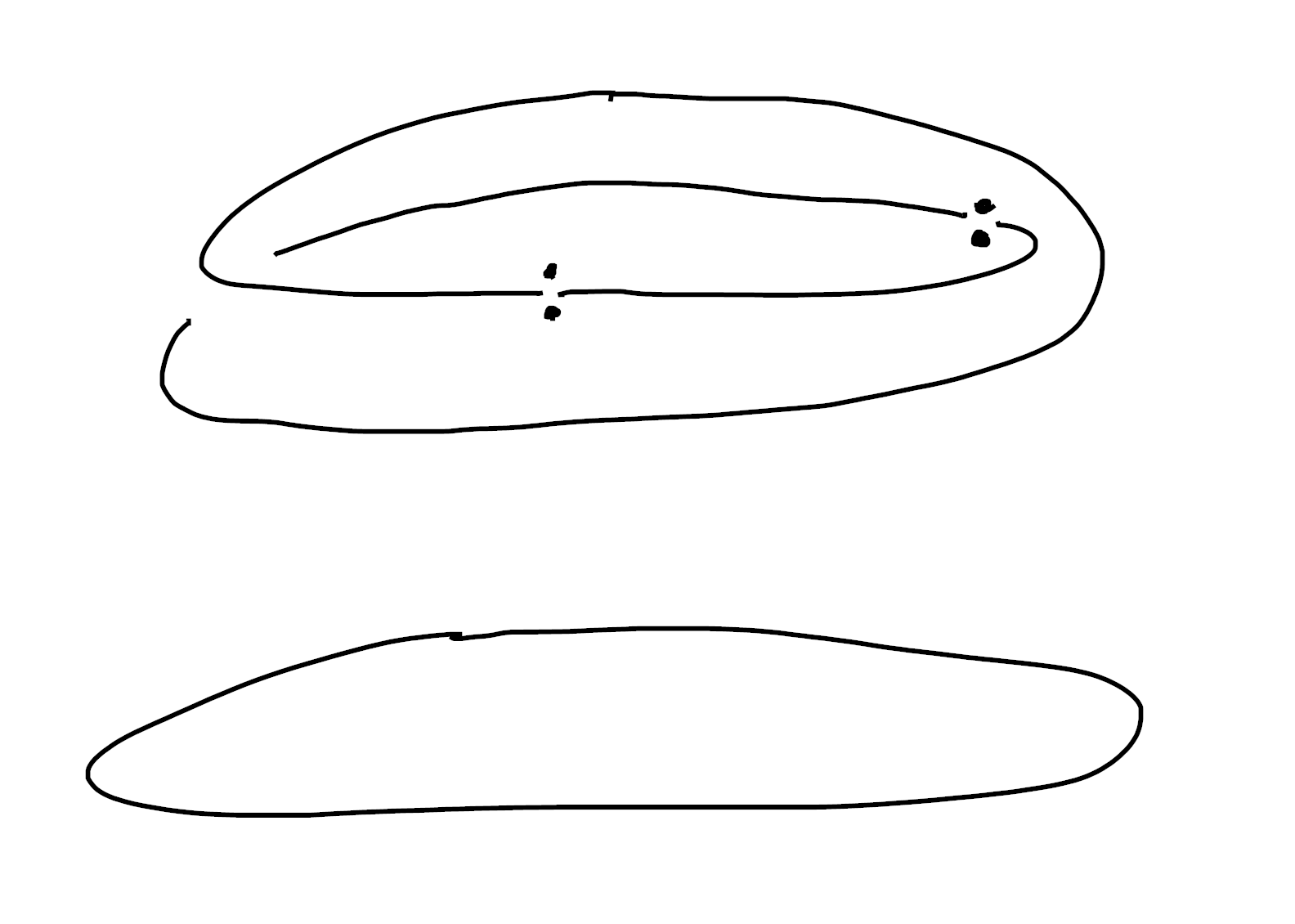
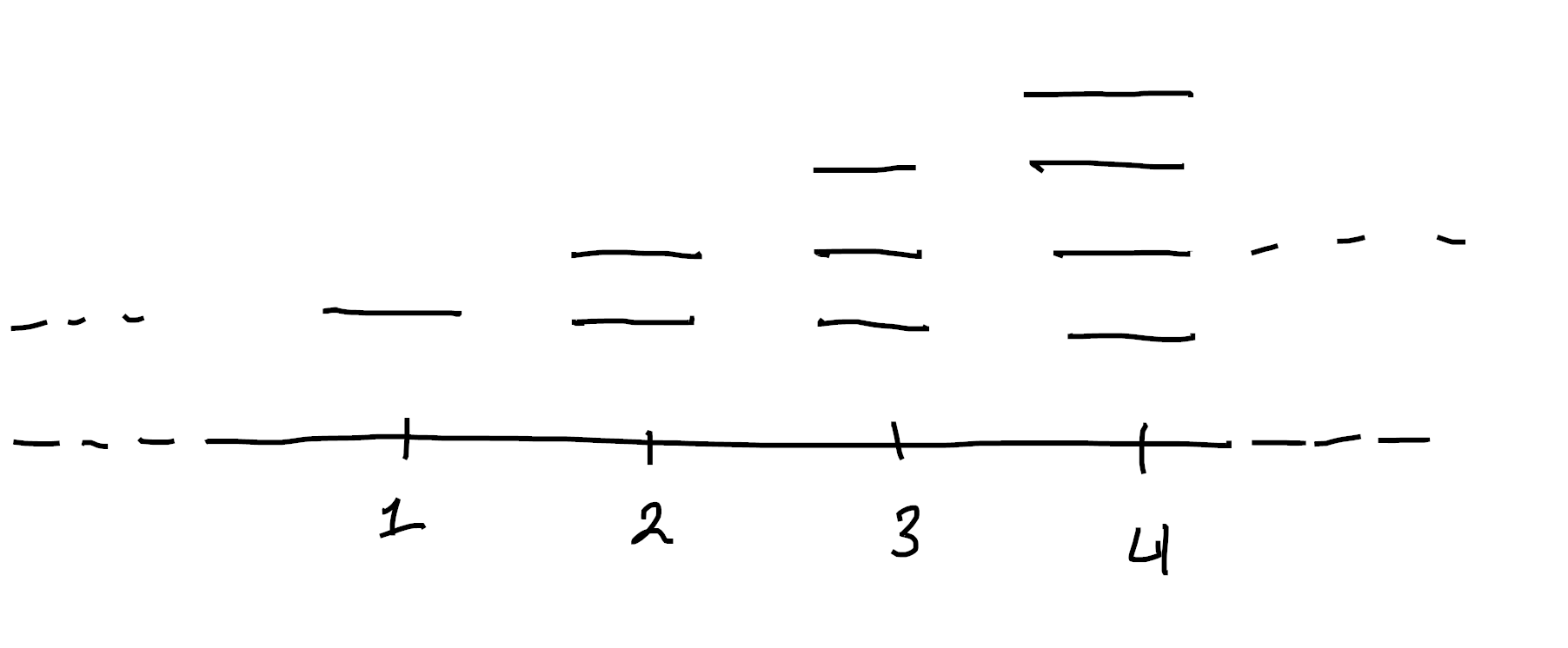
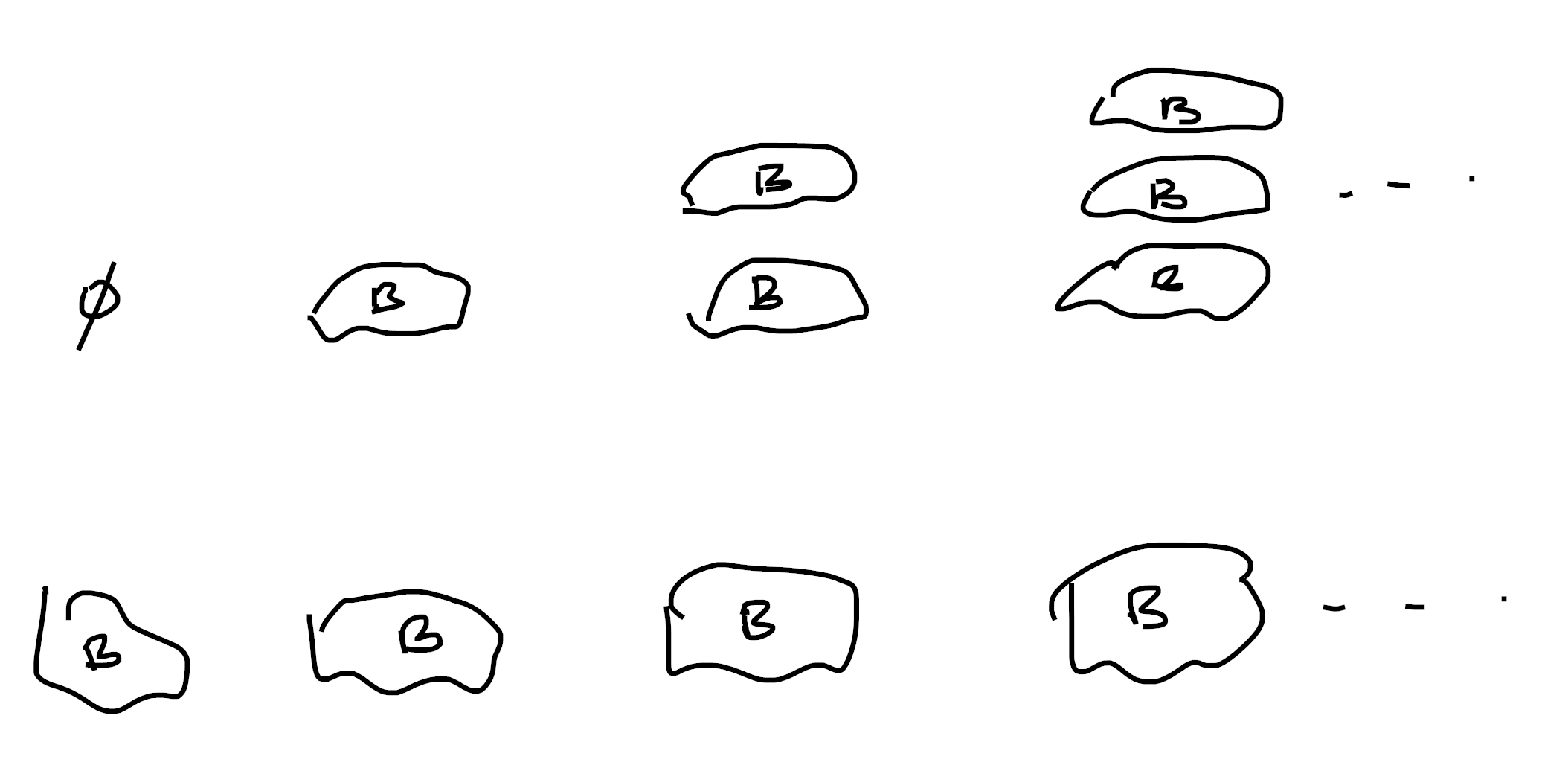
Kuratwoski finite sets can be shockingly complicated! Especially in contrast to the relatively tame bishop finite sets. For example, consider $B = \mathbb{R}$ with a skyscraper sheaf at every integer¹⁵:

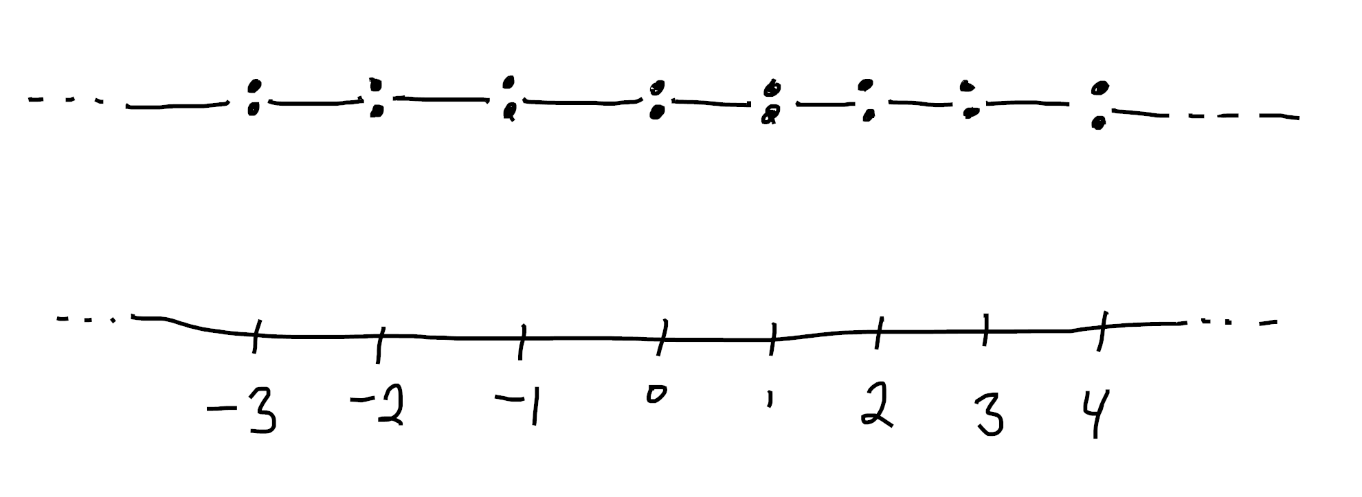
This space is kuratowski finite in $\mathsf{Sh}(\mathbb{R})$ (since it’s locally a quotient of $\mathbb{R} \sqcup \mathbb{R}$), but it has continuum many global sections! Indeed, we can choose either the top or the bottom point at every integer.

Since even the choice of $[n]$ is local, we can change the size of the fibres as long as they’re all finite!

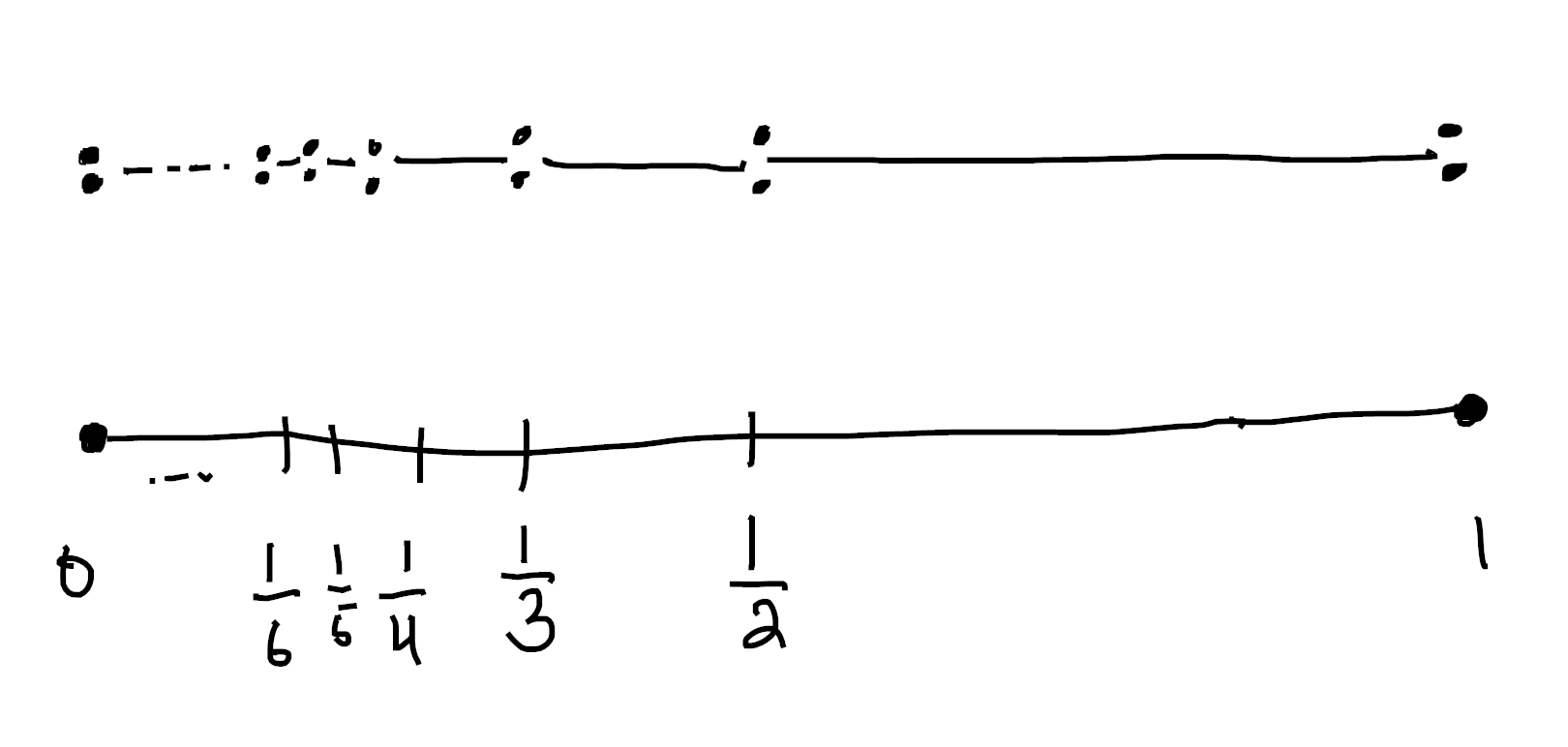
In fact, on mastodon (here and here), Antoine Chambert-Loir and Oscar Cunningham pointed out that you can do even weirder things. For instance, the set \(\{\frac{1}{n} \mid n \in \mathbb{N} \} \cup \{ 0 \}\) is closed in $[0,1]$. So its complement is open, and we can glue two copies of $[0,1]$ together along it! This gives us a kuratowski finite object which nonetheless has infinitely many sections in every neighborhood of $0$¹⁶!

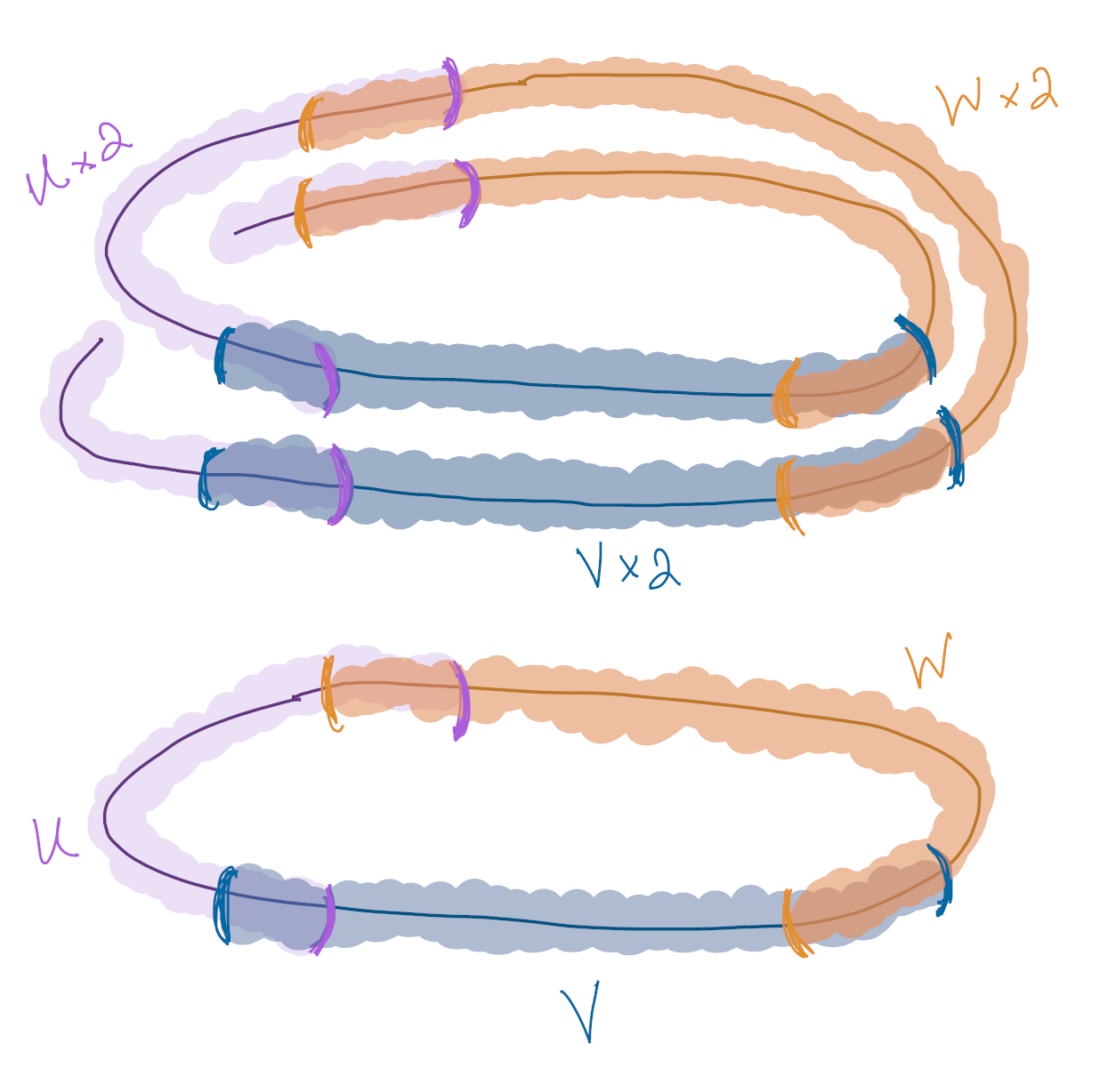
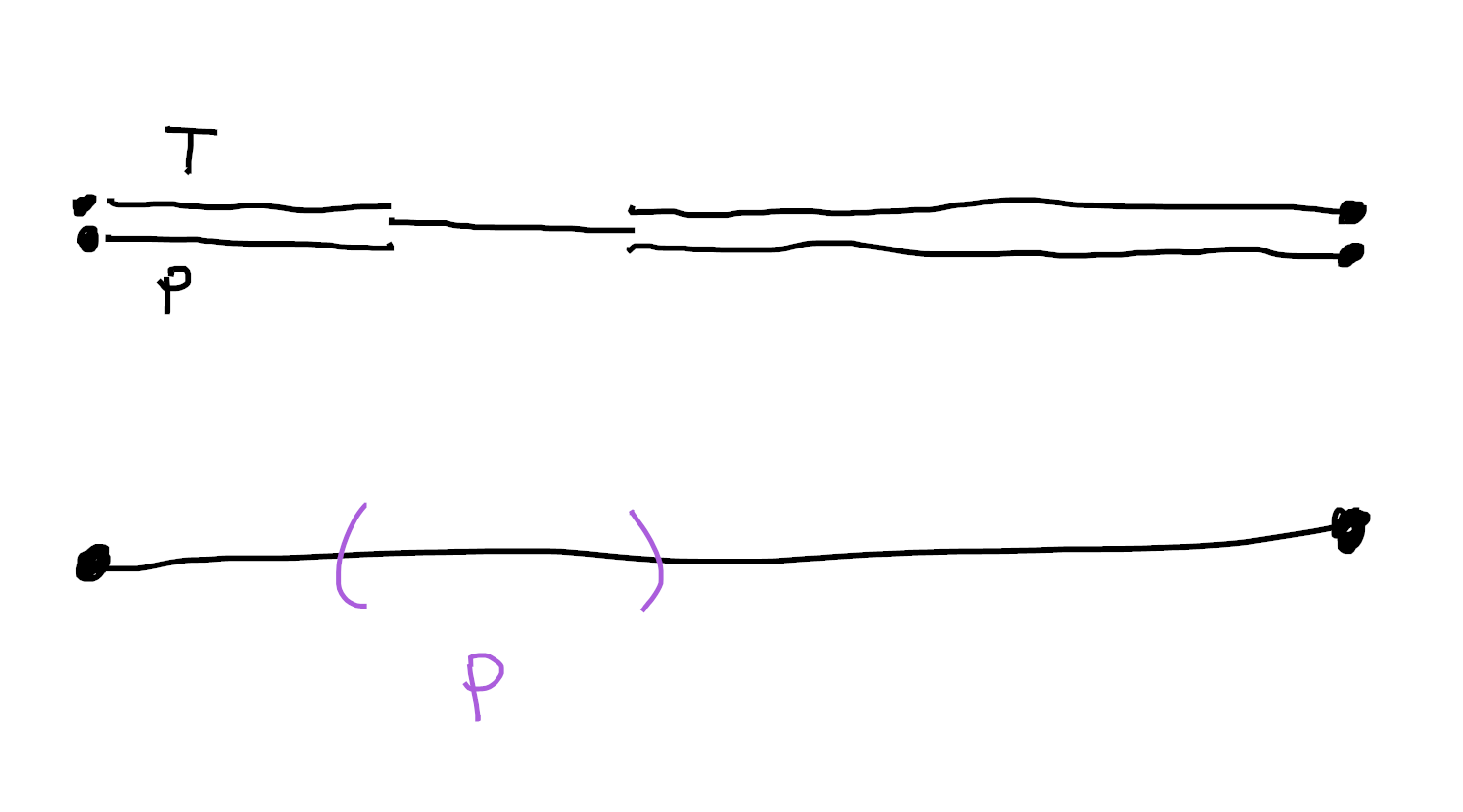
Finally, let’s talk about subfinite sets. These are locally subobjects of cardinals, so are much easier to visualize again!

A subobject of a cardinal is just a disjoint union of open subsets of $B$:

So a subfinite set has to locally look like these. Keep in mind, though, that like kuratowski finite sets, the choice of $[n]$ is made locally. So we can have something like this:

In particular, we see that the fibres of a subfinite set don’t need to be globally bounded! So, perhaps surprisingly, a subfinite set does not need to be a subobject of a bishop finite set!

As we’ve come to expect, the existential quantifier gives us the ability to twist.

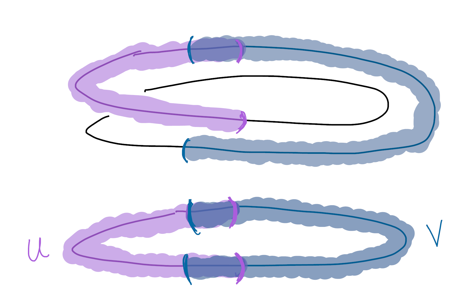
As subobjects of decidable objects, we see these inherit decidable equality. However, while bishop and kuratowski finite objects are all either empty or inhabited, subfinite sets don’t need to be! For an easy example, consider

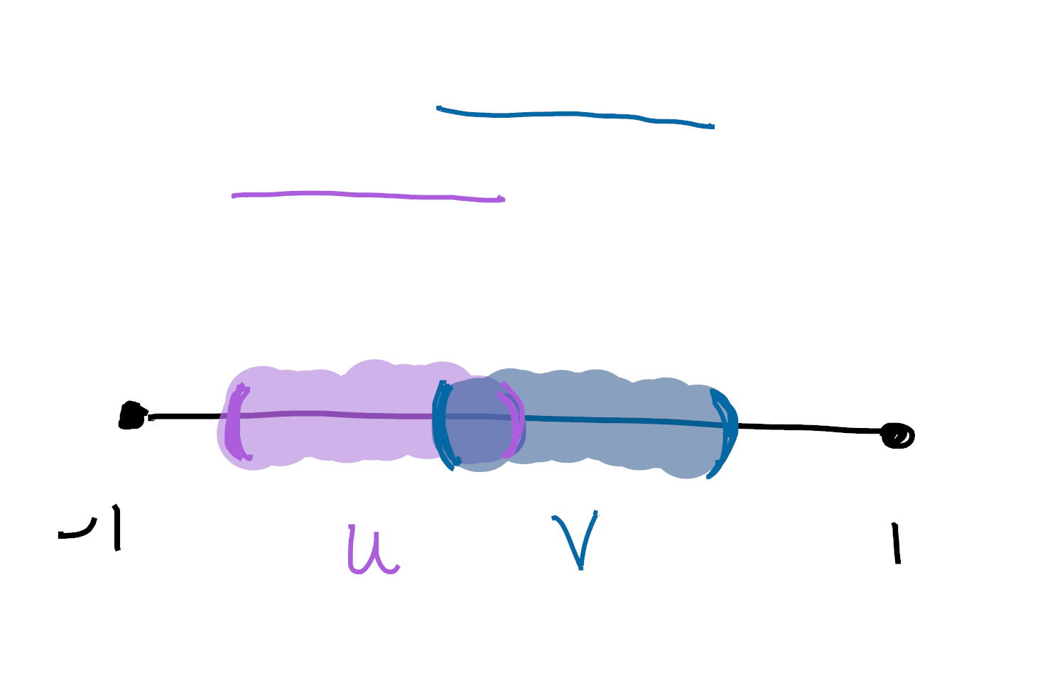
Here the truth value of $\exists x : X$ is $U \cup V$, and the truth value of $X = \emptyset$ is $\text{int}(U^c \cap V^c)$. (Do you see why?)

---

An aside on decidable equality

This isn’t technically about visualizing etale spaces, but I was thinking about it while writing this post, and I think it fits well enough to include. If nothing else, it’s deifnitely interesting enough to include!

If you’re really paying attention, you’ll notice the “easy exercise” about analytic continuation didn’t actually use any aspects of finiteness. Indeed, we can prove the following (very general) theorem:

$\ulcorner$ The equivalence of $1$ and $2$ was the earlier exercise, and you can find a proof below it under a fold/

To check the equivalence of $2$ and $3$, we look at “decidable equality”, that $\forall f,g : \mathcal{F} . (f=g) \lor (f \neq g)$.

Externally, this says that for every $U$, for every pair of local sections $f,g \in \mathcal{F}(U)$, there’s an open cover \(\{U_\alpha\}\) so that on each member of the cover \(f \! \upharpoonright_{U_\alpha}\) and \(g \! \upharpoonright_{U_\alpha}\) are either everywhere equal or everywhere unequal.

Clearly if $\mathcal{F}$ has analytic continuation then $\mathcal{F}$ has decidable equality. Indeed using local connectedness of $B$ we can cover $U$ by connected opens. By analytic continuation we know that on each connected piece either $f=g$ everywhere or nowhere, as desired.

Conversely, say $\mathcal{F}$ has decidable equality. Fix a connected $U$ and sections $f,g \in \mathcal{F}(U)$ which have the same stalk at some point $b \in U$. By decidable equality, there’s an open cover \(\{ U_\alpha \}\) of $U$ where on each member of the cover $f=g$ holds everywhere or nowhere. Recall that since $U$ is connected, for any two opens in the cover $U_\alpha$ and $U_\beta$ we can find a finite chain $U_\alpha = U_0, U_1, U_2, \ldots, U_n = U_\beta$ of opens in our cover where each $U_i$ intersects $U_{i+1}$.

Then for any $U_\beta$ in the cover, fix such a chain from $U_0 \ni b$ to $U_\beta$. By decidable equality we know $f=g$ on $U_0$. So for the point in $U_0 \cap U_1$ we know $f=g$, and by decidable equality again we learn $f=g$ on $U_1$. Proceeding in this way we learn $f=g$ on the whole of $U_\beta$.

Thus $f=g$ on every member of the cover, so on the whole of $U$, and so $\mathcal{F}$ satisfies analytic continuation. $\lrcorner$

If you’ve internalized this, it makes it geometrically believable that a decidable kuratowski finite set is actually bishop finite! I think it’s fun to see this fact both syntactically (reasoning in the internal logic) and semantically (reasoning about bundles), so let’s see two proofs!

First, a syntactic proof:

$\ulcorner$ Say $f : [n] \twoheadrightarrow X$. Then we note for each $x:X$ the predicate $\varphi(k) \triangleq f(k) = x$ on $[n]$ is decidable since $X$ has decidable equality. Thus it gives an inhabited decidable subset of $[n]$, which has a least element (Lemma D5.2.9(iii) in the elephant). Call such an element $g(x)$.

Note the image of $g$ is a complemented subset of $[n]$, since we can decide $k \in \text{im}(g)$ by checking if $k = g(f(k))$ using decidability of $[n]$. Then $\text{im}(g)$ is isomorphic to a cardinal (D5.2.3), $[m]$, and it’s easy to see that composing $g$ and $f$ with this isomorphism gives a bijection between $X$ and $[m]$. $\lrcorner$

And now a semantic proof:

$\ulcorner$ Say $\pi : E \twoheadrightarrow B$ is the etale space of a kuratowski finite object in $\mathsf{Sh}(B)$. So, locally, $E$ is the quotient of some $\coprod_n B$. Say also that $E$ is has decidable equality so that, locally, two sections of $E$ that agree somewhere must agree everywhere.

By refining our covers, then, we may fix an open cover \(\{U_\alpha\}\) of $B$ and epimorphisms \(\coprod_{n_\alpha} U_\alpha \to E \! \upharpoonright_{U_\alpha}\) so that two local sections on $U_\alpha$ either agree everywhere or nowhere. In particular, the $n_\alpha$ many components $f_i : U_\alpha \overset{i\text{th inclusion}}{\longrightarrow} \coprod_{n_\alpha} \to E$ are pairwise either have the same image or disjoint images. Choosing exactly one $f_i$ for each possible image (the least $i$ that works, say) we see that actually $\pi^{-1}(U_\alpha)$ is homeomorphic to the disjoint union of copies of $U_\alpha$ so that $E$ is actually a covering space, and thus represents a bishop finite object. $\lrcorner$

---

Which Finite to Use?

Constructively, bishop and kuratowski finiteness encode two aspects of finiteness which are conflated in the classical finite world. Bishop finite sets are those which admit a cardinality. They’re in bijection with some $[n]$, and so have a well defined notion of size. Kuratowski finite sets, in contrast, are those equipped with an enumeration. You can list all the elements of a kuratowski finite set.

Of course, knowing how to biject a set $X$ with a set $[n]$ always tells you how to enumerate $X$. But constructively knowing how to enumerate $X$ doesn’t tell you how to biject it with some $[n]$! As we saw earlier, the problem lies with removing duplicates. It’s worth taking a second to visualize a kuratowski finite set that isn’t bishop finite, and convince yourself that the question “is this a duplicate element” can have more subtle answers than just “yes” or “no”. This makes it impossible to remove the duplicates.

This bifurcation might feel strange at first, but in some squishy sense it happens classically too once you start working with infinite sets. Indeed in set theory the notion of finiteness bifurcates into cardinals, which have a defined notion of “size”, and ordinals, which have a defined notion of “order” (kind of like an enumeration… if you squint).

So when you’re working constructively, ask why you’re using finiteness. Do you really need to know that something literally has $n$ elements for some $n$? Or is it enough to know that you can put the elements in a finite list? Does it matter if your list has duplicates? These questions will tell you whether bishop finiteness or kuratowski finiteness is right for your purposes.

Subfiniteness, which amounts to being contained in some $[n]$, I find to be less useful “in its own right”. Instead, if you’re able to prove a result for bishop finite objects, it’s worth asking if you can strengthen that to a proof for subfinite ones!

In any case, as long as we work with decidable things, these notions all coincide. As we saw earlier, a decidable quotient of a bishop finite set (that is, a decidable kuratowski finite set) is again bishop finite. Similarly, a complemented subset of a bishop finite set is finite (this is lemma D5.2.3 in the elephant, but it’s not hard to see yourself). So if you’re working in a context where everything is decidable, finite sets work exactly as you would expect! This is part of why constructive math doesn’t have much to say about combinatorics and algebra. Most arguments are already constructive for decidable finite sets (which is what you’re picturing when you picture a finite set and do combinatorics to it). Sometimes you can push things a bit farther though, and this can be interesting. See, for instance, Andreas Blass’s paper on the Constructive Pigeonhole Principle.

---

Another blog post done! I’m writing this on a train to Odense right now, and once I get to my room I’ll draw all the pictures and post it.

Hopefully this helps demystify the ways in which constructive math might look strange at first. Once again the seemingly bizarre behavior is explained by its vastly greater generality! When you first learn that a subset of a (bishop) finite set need not be (bishop) finite, it sounds so strange as to be unusable! But once you learn that this is an aspect of “everywhere definedness” in a space of parameters (read: the base space) it becomes much more palatable.

Thanks, as always, for hanging out. Try to keep cool during this summer heat (though it’s actually really pleasant in Denmark right now), and I’ll see you all soon ^_^.

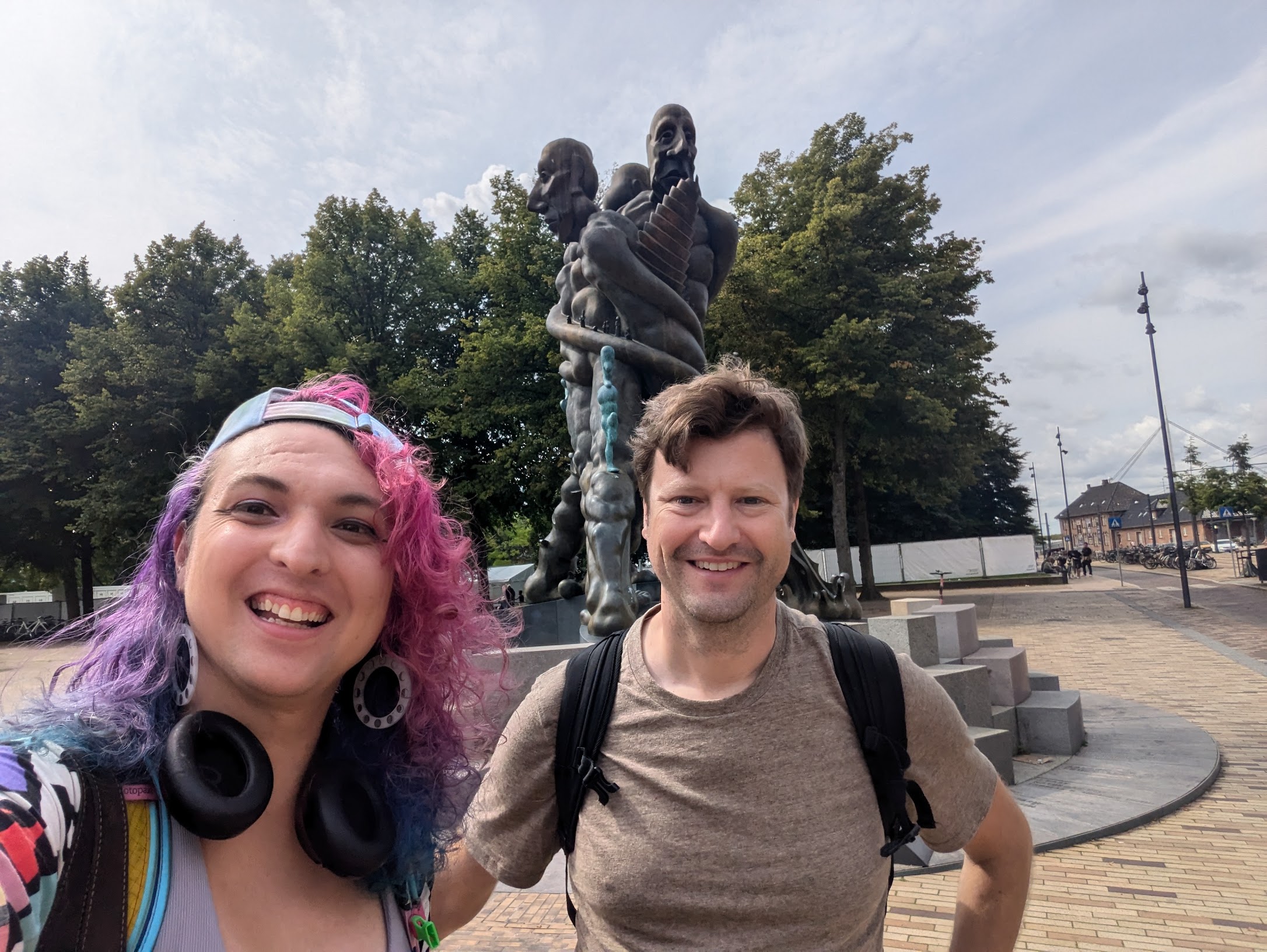
Here’s a picture of me and Peter right after we got off the train:

---