Analytic Combinatorics -- A Worked Example

08 Apr 2025 - Tags: sage

Another day, another blog post that starts with “I was on mse the other day…”. This time, someone asked an interesting question amounting to “how many unordered rooted ternary trees with $n$ nodes are there, up to isomorphism?”. I’m a sucker for these kinds of combinatorial problems, and after finding a generating function solution I wanted to push myself to get an asymptotic approximation using Flajolet–Sedgewick style analytic combinatorics! I’ve never actually done this before, so I learned a lot, and I want to share some of the things I learned – especially how to do this stuff in sage!

Now, you might be thinking – didn’t you write a very similar blog post three years ago? Yes. Yes I did. Did I also completely forget what was in that post? Yes. Yes I did, haha. For some reason I was getting it mixed up with this other post from even more years ago, which isn’t nearly as relevant. Thankfully it didn’t matter much, since I’m fairly sure what I wanted to do wouldn’t work in the framework of that post anyways, and now I have a better idea of what this machinery is actually doing which is really exciting (since I’ve been wanting to understand this stuff for years).

Let’s start with a warmup problem! How might we count the number of rooted ordered ternary trees with $n$ nodes?

These are the kinds of “ternary trees” that you might remember from a first class on algorithms and data structures. Such a tree is either a leaf or an internal node with 1,2, or 3 children. Crucially these children come with an order, because the datatype keeps track of which child is on the left/right (in the case of 2 children) or on the left/middle/right (in the case of 3 children). After all, from a CS perspective, we need to remember this in order to traverse the tree!

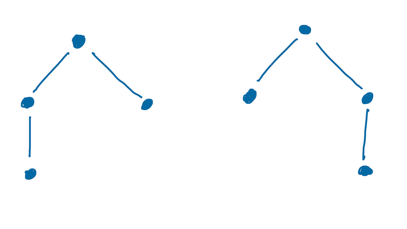
This means that the following two trees are distinct for our purposes, even though they’re isomorphic as graphs:

In a functional programming language, you might describe this datatype by

T z = Leaf z
    | Unary z (T z)
    | Binary z (T z) (T z) 
    | Ternary z (T z) (T z) (T z)

and this translates immediately to give a functional equation for the generating function of $t_{n}$ , which counts the number of rooted ordered ternary trees with $n$ nodes:

T (z) = z + z T + z T^{2} + z T^{3}

We can rearrange this as

z = \frac{T}{1 + T + T^{2} + T^{3}}

so that we can compute the power series expansion of $T$ by lagrange inversion:

xxxxxxxxxx
 
R.<z> = QQbar[[]] # power series ring
T = (z/(1 + z + z^2 + z^3)).reverse()
show(T.O(10))

Incredibly, this agrees with A036765, which is the “number of ordered rooted trees with n non-root nodes and all outdegrees <= three”, as we hoped!

You might reasonably ask if there’s a closed form for these numbers, and this is too much to ask for (indeed, it’s already too much to ask for a closed form for fibonacci numbers, and this is more complicated). But like the fibonacci numbers, we can come up with an excellent approximation:

t_{n} = [z^{n}] T \approx C \frac{(3.6107 \dots)^{n}}{n^{3 / 2}} (1 \pm O (\frac{1}{n}))

where $C = \frac{(0.8936 \dots)}{2 \sqrt{π}}$ is a constant.

Indeed, this gives fantastic results! Let’s plot the ratio of this approximation to the true value so we can see just how good this approximation gets as $n$ gets large. Note that it respects the promised big-oh error bound too!

xxxxxxxxxx
 
def actual(n,N):
    R.<z> = PowerSeriesRing(QQbar, default_prec=N)
    T = (z/(1 + z + z^2 + z^3)).reverse()
    return T.coefficients()[n-1:]
​
def approx(n,N): 
    # very very magic
    C = 0.8936373911078061 / (2 * sqrt(pi))
    w = 3.610718613276040
    return [(C * w^k * (1/k^1.5)).n() for k in range(n,N+1)]
​
show(html("Plot the error ratios in the range [n,N]"))
@interact
def _(n=input_box(100, width=20, label="$n$"),
      N=input_box(120, width=20, label="$N$"),
      auto_update=False): 
​
    actuals = actual(n,N)
    approxs = approx(n,N)
    ratios  = [(actuals[i]/approxs[i]) for i in range(N+1-n)]
    show(html("ratio at n={}: {}".format(n, ratios[0])))
    show(html("ratio at N={}: {}".format(N, ratios[-1])))
​
    text_options = {'horizontal_alignment': 'right',
                    'vertical_alignment': 'bottom', 
                    'fontsize': 'large'}
​
    G = Graphics()
    G += scatter_plot([(n+i,r) for (i,r) in enumerate(ratios)])
    G += plot(1, (x,n,N))
    G += plot(1-1/x, (x,n,N))
    G += text('$y = 1$', (N, 1), **text_options)
    G += text('$y = 1-1/x$', (N, 1-1/N), **text_options)
​
    G.show()

This is extremely cool, but where the hell did this approximation come from?

The answer is called Singularity Analysis, and can be found in Chapter 2 Section 3 of Melczer’s excellent An Invitation to Analytic Combinatorics, or Chapters VI and VII of Flajolet and Sedgewick’s tome. See especially Theorem VII.3 on pg 468.

Like seemingly every theorem in complex analysis, this is basically an application of the Residue Theorem. I won’t say too much about why it works, but I’ll at least gesture at a proof. You can read the above references if you want something more precise.

First, we recall

t_{n} = \frac{1}{2 π i} \int_{C} \frac{T}{z^{n + 1}} d z

where $C$ is any contour containing the origin inside a region where $T$ is holomorphic.

Then we draw the most important picture in complex analysis:

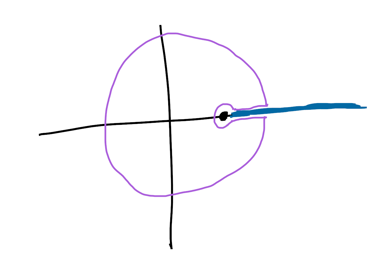
Here the obvious marked point is our singularity $ω$ , and we’ve chosen a branch cut for $T$ (shown in blue¹) so that $T$ is holomorphic in the region where the pink curve lives. We’ll estimate the value of this integral by estimating the contribution from the big circle, the little circle, and the two horizontal pieces².

It turns out that the two horizontal pieces basically contribute $O (1)$ amount to our integral, so we ignore them. Since the big circle is compact, $T$ will attain a maximal value on it, say $M$ . Then the integral along the big circle (of radius $ω + ϵ$ , say) is bounded by $2 π (ω + ϵ) \frac{M}{(ω + ϵ)^{n + 1}} = O ((ω + ϵ)^{- n})$

To estimate the integral around the little circle, it would be really helpful to have a series expansion at $ω$ since we’re staying really close to it… Unfortunately, $ω$ is a singular point so we don’t have a taylor series, but fortunately there’s another tool for exactly this job: a Puiseux Series!

I won’t say much about what these are, especially since Richard Borcherds already put out such a great video on the topic. What matters is is that Sage can compute them for us³, so we can actually get our hands on the approximation!

We compute the integral⁴ around the little circle to be roughly:

\begin{aligned} \frac{1}{2 π i} \int \frac{T}{z^{n + 1}} d z & \overset{(1)}{\approx} \frac{1}{2 π i} \int \frac{c_{α} (1 - \frac{z}{ω})^{α}}{z^{n + 1}} d z \\ \overset{(2)}{=} \frac{1}{2 π i} \int \frac{c_{α} \sum_{k} (\binom{α}{k}) (\frac{- z}{ω})^{k}}{z^{n + 1}} d z \\ \overset{(3)}{=} c_{α} (\binom{α}{n}) \frac{(- 1)^{n}}{ω^{n}} \end{aligned}

In step $(1)$ we approximate $T$ by the first term of its puiseux series, in step $(2)$ we apply the generalized binomial theorem, so that in step $(3)$ we can apply the residue theorem to realize this integral as the coefficient of $z^{- 1}$ in our laurent expansion.

This gives us something which grows like $\tilde{O} (ω^{- n})$ , dominating the contribution $O ((ω + ϵ)^{- n})$ from the big circle, so that asymptotically this is the only term that matters. If we were more careful to keep track of the big-oh error for the puiseux series for $T$ we could easily sharpen this bound⁵ to see

t_{n} = c_{α} (\binom{α}{n}) \frac{(- 1)^{n}}{ω^{n}} (1 + O (\frac{1}{n}))

This looks a bit weird with the $(- 1)^{n}$ , but remember that $(\binom{α}{n})$ also alternates sign. Indeed, asymptotics for $(\binom{α}{n})$ are well known so that we can rewrite this as

t_{n} = \frac{c_{α}}{Γ (- α)} \frac{ω^{- n}}{n^{α + 1}} (1 + O (\frac{1}{n}))

Which finally shows us where our magic numbers came from! Sage happily tells us that the dominant singularity for $T$ is at $ω = (0.2769 \dots)$ and that a puiseux expansion for $T$ at $ω$ is

T \approx (0.65 \dots) - (0.8936 \dots) (1 - z / ω)^{1 / 2} + \dots

so that for us $α = 1 / 2$ , and $C_{1 / 2} = - (0.8936 \dots)$ .

Finally, since $Γ (- 1 / 2) = - 2 \sqrt{π}$ and $(0.2769 \dots)^{- 1} = (3.6107 \dots)$ we see

t_{n} = \frac{(0.8936 \dots)}{2 \sqrt{π}} \frac{(3.6107 \dots)^{n}}{n^{3 / 2}} (1 + O (\frac{1}{n}))

as promised!

Indeed, here’s how you could actually get sage to do all this for you!

xxxxxxxxxx
 
# at time of writing the abelfunctions package
# isn't installed on sagecell, so you'll need to 
# run this locally if you want to play with it
import abelfunctions
​
# to compute the discriminant we need P to be a 
# polynomial whose coefficients are polynomials.
R.<z> = QQbar[]
S.<T> = R[]
​
# our defining polynomial. 
# we want to solve for T as a function of z
P = z*T^3 + z*T^2 + (z-1)*T + z
​
# following Example 2.12 in Melczer,
# we compute the dominant singularity w. 
w = min([r for (r,_) in P.discriminant().roots() if r != 0], 
        key=lambda r: r.abs())
​
# to work with abelfunctions we need P 
# to be a polynomial in two variables
R.<z,T> = QQbar[]
P = R(P)
​
# compute the puiseux expansion for T at w. 
# I know from trial and error that the correct 
# branch to pick is entry [1] in the list. You 
# just need to check which one gives you 
# positive real coefficients for T at 0.
s = abelfunctions.puiseux(P,w)[1]
c = -sqrt(-s.x0/s.xcoefficient)

As a fun exercise, you might modify this code (using s.add_term()) to compute a longer puiseux series and get asymptotics valid up to a multiplicative error of $O (\frac{1}{n^{2}})$ for the number of rooted ternary trees.

Try modifying the previous code block to see that our current approximation is not accurate to $O (\frac{1}{n^{2}})$ , and then check that your approximation is!

Ok, now that we understand the warmup, let’s get to the actual problem!

How many unordered rooted ternary trees are there, up to isomorphism?

Now we’re counting up to graph isomorphism, so that our two trees

are now considered isomorphic. It’s actually much less obvious how one might pin down a generating function for something like this, but the answer, serendipitously, comes from Pólya-Redfield counting! If this is new to you, you might be interested in my recent blog post where I talk a bit about one of its corollaries. Today, though, we’ll be using it in a much more sophisticated way.

Say you have a structure $X$ acted on by a group $G$ and a collection $C$ of “colors”. How can we count the number of ways to give each $x \in X$ a color from $C$ , up to the action of $G$ ?

We start by building the cycle index polynomial of the action $G ↷ X$ , which we call $P_{G} (x_{1}, \dots, x_{n})$ . Then we can plug all sorts of things into the variables $x_{i}$ in order to solve various counting problems. For example, if $C$ is literally just a finite set of colors, we can plug in $x_{1} = x_{2} = \dots = x_{n} = | C |$ to recover the expression from my recent blog post. But we can also do much more!

Say that $C$ is a possibly infinite family of allowable “colors”, each of a fixed “weight”. (For us, our “colors” will be trees, and the “weight” will be the number of nodes). Then we can arrange them into a generating function $F (t) = \sum c_{i} t^{i}$ , where $c_{i}$ counts the number of colors of weight $i$ ⁶. Then an easy argument (given in full on the wikipedia page) shows that $P_{G} (F (t), F (t^{2}), \dots, F (t^{n}))$ is a generating function counting the number of ways to color $X$ by colors from $C$ , counted up to the $G$ action, and sorted by their total weight⁷. Check out the wikipedia page for a bunch of great examples!

For us, we realize an unordered rooted ternary tree is either empty, or a root with 3 recursive children⁸. In the recursive case we also want to count up to the obvious $S_{3}$ action permuting the children, so by the previous discussion we learn that

T (z) = 1 + z P_{S_{3}} (T (z), T (z^{2}), T (z^{3}))

where $P_{S_{3}} (x_{1}, x_{2}, x_{3}) = \frac{1}{6} (x_{1}^{3} + 3 x_{1} x_{2} + 2 x_{3})$ is the cycle index polynomial for the symmetric group on three letters. Plugging this in we see

T (z) = 1 + \frac{z}{6} (T (z)^{3} + 3 T (z) T (z^{2}) + 2 T (z^{3}))

Now, how might we get asymptotics for $t_{n}$ using this functional equation?

First let’s think about how our solution to the warmup worked. We wrote $F (z, T) = 0$ for a polynomial $F$ , used the implicit function theorem to get a taylor series for $T$ at the origin, then got a puiseux series near the dominant singularity $ω$ which let us accurately estimate the taylor coefficients $t_{n}$ ⁹.

We’re going to play the same game here, except we’ll assume that $F$ is merely holomorphic rather than a polynomial. Because we’re no longer working with a polynomial, this really seems to require an infinite amount of data, so I’m not sure how one might get an exact solution for the relevant constants… But following Section VII.5 in Flajolet and Sedgewick we can get as precise a numerical solution as we like!

We’ll assume that the functions $T (z^{2})$ and $T (z^{3})$ are already known analytic functions, so that we can write $F (z, w) = - w + 1 + \frac{z}{6} (w^{3} + 3 T (z^{2}) w + 2 T (z^{3}))$ . This is an analytic function satisfying $F (z, T) = 0$ .

Now for a touch of magic. Say we can find a pair $(r, s)$ with both $F (r, s) = 0$ and ${\frac{\partial F}{\partial w} |}_{(r, s)} = 0$ … Then $F$ is singular in the $w$ direction at $(r, s)$ so this is a branch point for $T$ . Since both $F$ and $F_{w} = \frac{\partial F}{\partial w}$ vanish at $(r, s)$ the taylor series for $F$ at $(r, s)$ starts

F_{z} (r, s) (z - r) + \frac{1}{2} F_{w w} (r, s) (w - s)^{2}

Since we know $F (z, T)$ vanishes, we estimate up to smaller order terms

F_{z} (r, s) (z - r) + \frac{1}{2} F_{w w} (r, s) (T - s)^{2} = 0

so that a puiseux series for $T$ at $(r, s)$ begins

T = s \pm \sqrt{\frac{2 r F_{z} (r, s)}{F_{w w} (r, s)}} {(1 - \frac{z}{r})}^{1 / 2}

If we write $γ = \sqrt{\frac{2 r F_{z} (r, s)}{F_{w w} (r, s)}}$ and are slightly more careful with our error terms, the same technique from the warmup shows

t_{n} = \frac{γ}{Γ (- 1 / 2)} \frac{r^{- n}}{n^{3 / 2}} (1 + O (\frac{1}{n}))

See Flajolet and Sedgewick Theorem VII.3 on page 468 for a more careful proof of this theorem.

Now how do we use this? We can approximate $T$ by its taylor series at the origin, then numerically solve for the unique¹⁰ positive real solution to the system $F (r, s) = F_{w} (r, s) = 0$ using this approximation:

xxxxxxxxxx
 
# how far we taylor expand T. This controls the accuracy 
# of our approximation of (s,r).
# the sagecell times out if you make this too big, so you 
# might want to run this locally.
N = 5
​
# get the first n taylor coefficients for T
def approx(n):
    B = PolynomialRing(QQ, 't', n+1)
    t = B.gens()
    R.<z> = B[[]]
​
    # cycle index polynnomials
    S.<x1,x2,x3> = QQ[]
    P3 = (x1^3 + 3*x1*x2 + 2*x3)/6
​
    # to start, the taylor coefficients of T are variables
    T = sum([t[i] * z^i for i in range(n)]) + O(z^n)
​
    lhs = T
    rhs = 1 + z*P3.subs(x1=T(z), x2=T(z^2), x3=T(z^3))
​
    # formally expand out the rhs and set the coefficients 
    # equal to each other. This gives a recurrence relation 
    # for t[n] in terms of the t[i] for i<n. 
    # Then we solve this recurrence via groebner bases, 
    # which is extremely fast.
    I = B.ideal([lhs.coefficients()[i] - rhs.coefficients()[i] 
                 for i in range(n)])
​
    # add all our solved coefficients back together to 
    # get an approximation for T
    return sum([I.reduce(t[i])*z^i for i in range(n)]) + O(z^n)
​
z,w = var('z,w')
T = SR(approx(N).truncate())
F = -w + 1 + (z/3)*T.subs(z=z^3) + (z/2)*T.subs(z=z^2)*w + (z/6)*w^3
​
eqns = [diff(F,w)==0, F==0]
solns = [[a.rhs(), b.rhs()] for [a,b] in solve(eqns,[z,w])]
realSolns = [[a,b] for [a,b] in solns if a in RR and b in RR]
[r,s] = realSolns[0]
​
show(html("$r={}$".format(r)))
show(html("$s={}$".format(s)))
​
gamma = -sqrt(2*r*diff(F,z).subs(z=r,w=s)/diff(F,w,2).subs(z=r,w=s))
​
show(html("$\\gamma={}$".format(gamma)))

If we run this code locally with $N = 20$ , we get the approximation

\begin{aligned} r & \approx 0.3551817478731632 \\ s & \approx 2.1174205967276225 \\ γ & \approx - 1.8358222405236164 \end{aligned}

so that we expect

t_{n} \approx \frac{(1.835 \dots)}{2 \sqrt{π}} \frac{(0.355 \dots)^{- n}}{n^{3 / 2}}

and indeed this seems to work really well! Our taylor expansion for $T$ agrees with A000598, as we expected, and comparing our approximation to our taylor expansion gives:

xxxxxxxxxx
 
r = 0.3551817478731632
s = 2.1174205967276225
gamma = -1.8358222405236164
​
def approx(n):
    return (gamma / (-2 * sqrt(pi))) * (r^(-n) / n^(3/2))
​
def approxList(n,N):
    return [approx(k) for k in range(n,N)]
​
def actualList(n,N):
    B = PolynomialRing(QQ, 't', N+1)
    t = B.gens()
    R.<z> = B[[]]
​
    S.<x1,x2,x3> = QQ[]
    P3 = (x1^3 + 3*x1*x2 + 2*x3)/6
​
    T = sum([t[i] * z^i for i in range(N)]) + O(z^N)
​
    lhs = T
    rhs = 1 + z*P3.subs(x1=T(z), x2=T(z^2), x3=T(z^3))
​
    I = B.ideal([lhs.coefficients()[i] - rhs.coefficients()[i] 
                 for i in range(N)])
​
    return [I.reduce(t[i]) for i in range(n,N)]
    
show(html("Plot the error ratios in the range [n,N]"))
show(html("This is likely to time out if you make N too large online,"))
show(html("so you might want to play around with it locally instead!"))
@interact
def _(n=input_box(10, width=20, label="$n$"),
      N=input_box(30, width=20, label="$N$"),
      auto_update=False): 
​
    actuals = actualList(n,N)
    approxs = approxList(n,N)
    ratios  = [actuals[i]/approxs[i] for i in range(N-n)]
    show(html("ratio at n={}: {}".format(n, ratios[0].n())))
    show(html("ratio at N={}: {}".format(N, ratios[-1].n())))
​
    text_options = {'horizontal_alignment': 'right',
                    'vertical_alignment': 'bottom', 
                    'fontsize': 'large'}
​
    G = Graphics()
    G += scatter_plot([(n+i,r) for (i,r) in enumerate(ratios)])
    G += plot(1, (x,n,N))
    G += plot(1-1/x, (x,n,N))
    G += text('$y = 1$', (N, 1), **text_options)
    G += text('$y = 1-1/x$', (N, 1-1/N), **text_options)
​
    G.show()

I’m pretty proud of this approximation, so I think this is a good place to stop ^_^.

As a fun exercise, can you write a program that outputs the number of cyclic rooted ternary trees on $n$ vertices? For these we consider two trees the same if they’re related by cyclicly permuting their children. Compare your solution to A000625

For bonus points, can you check that the number of such trees is, asymptotically,

t_{n} = (0.34630 \dots) \frac{(3.2871 \dots)^{n}}{n^{3 / 2}}

Wow! It’s been super nice to be writing up so many posts lately! Like I said in one of my other recent posts, I’ve had a lot of time to think about more bite sized problems and mse stuff while waiting for my DOI generating code to run, so I’ve had more things that felt quick to write up on my mind.

My research is actually going quite well too! I have a few interesting directions to explore, and at least one project that might be wrapping up soon. Of course when that happens I’ll be sure to talk about it here, and I’m still planning out a series on fukaya categories, hall algebras, skein algebras, and more! That’s a pretty long one, though, so it’s easy for me to deprioritize, haha.

It’s already heating up in Riverside, consistently in the 80s (Fahrenheit), so I can really feel the summer coming. I’m enjoying the sunny days, though, and it’s been nice to spend time working outside and under trees.

Thanks for hanging out, all! Take care of each other, and I can’t wait to chat soon ^_^.

Just like $w = \sqrt{z}$ , a solution to $w^{2} = z$ has branches, so too does $T$ , a solution to $T = z + z T + z T^{2} + z T^{3}$ . ↩
Really these are circles with a little arc cut out, say by integrating from $ϵ$ to $2 π - ϵ$ … But we’ll end up taking $ϵ \to 0$ and we’re all friends here, so let’s not worry about it. ↩
Though at time of writing you need the abelfunctions package to do it. There is a builtin implementation of puiseux series, but it won’t actually compute a series expansion for you. ↩
Thanks to Shane and Raj for helping me work this out! ↩
Of course, it’s easy to see how to extend this technique to get better asypmtotics. The first approach is to just keep more terms of the puiseux series of $T$ at $ω$ . Then apply the generalized binomial formula multiple times for each term you kept.

You can also do better by keeping track of more of the singularities. Build a contour with multiple keyholes in order to get sharper lower order asymptotics:

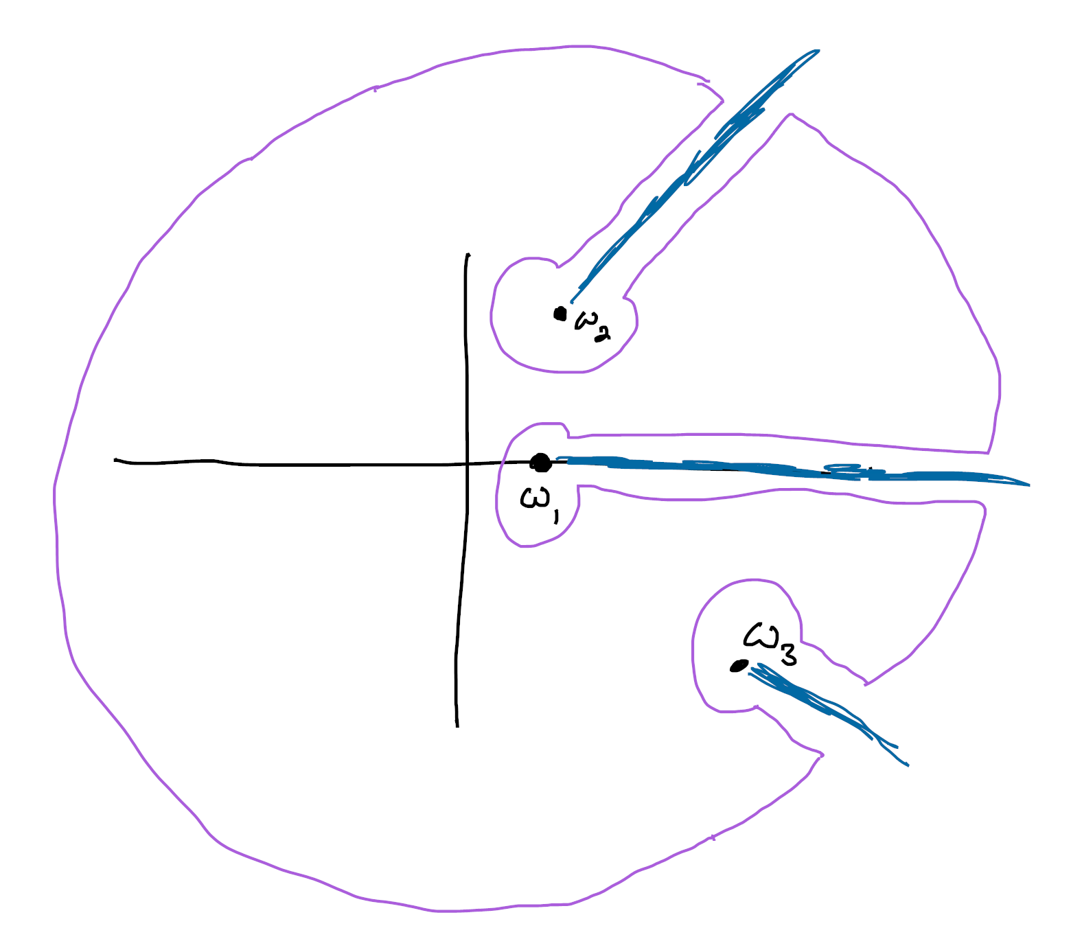
Of course, you can also combine these approaches to keep track of both more singularities and more puiseux coefficients at each singularity. ↩
In fact we can push things even farther and work with multivariate generating functions, but we won’t need that here. ↩
This is why we plug $F (t^{k})$ into $x_{k}$ . Because $x_{k}$ is responsible for $k$ -cycles, so we choose a single color for each $k$ cycle, but we have to count it $k$ -many times towards our total weight. See the proof on the wikipedia page for more information! ↩
This actually isn’t the version of the recurrence I used in my mse answer. There I used the convention that a rooted tree had to be nonempty, since… you know… it has a root.

But allowing possibly empty trees makes the recurrence much simpler, which in turn allows for much easier to analyze asymptotics. Hilariously this exact example is on the wikipedia page for the Pólya-Redfield theorem, which could have saved me a lot of time writing up that answer.

I was a bit worried at first about doing these asymptotics by myself, since this was my first serious attempt at using analytic combinatorics, but serendipitously this exact example was also worked out in Flajolet and Sedgewick VII.5, though slightly more tersely than I would have liked, haha. ↩
Officially we have to check that the choice of puiseux series matches up with our choice of taylor series (since there’s multiple branches to our function). But this is easy to arrange for us by choosing the branch of the puisuex series that leads to all our coefficients being positive reals. If you want to do this purely analytically you need to solve a “connection problem”. See figure VII.9 in Flajolet and Sedgewick, as well as the surrounding text. ↩
Under mild technical conditions this pair $(r, s)$ is unique. See Flajolet and Sedgewick Theorem VII.3. ↩