How to Explicitly Compute Charts for a Levelset Submanifold

20 Jun 2025

While doing a computation with my friend Shane the other day, we realized we needed to explicitly compute a local chart near the identity of $S{L}_2(\mathbb{R})$. It took us longer than I’d like to admit to figure out how to do this (especially since it’s so geometrically obvious in hindsight), and so I want to write down the process for future grad students looking to just do a computation! If you want to see what Shane and I were actually interested in, you can check out the main post here.

---

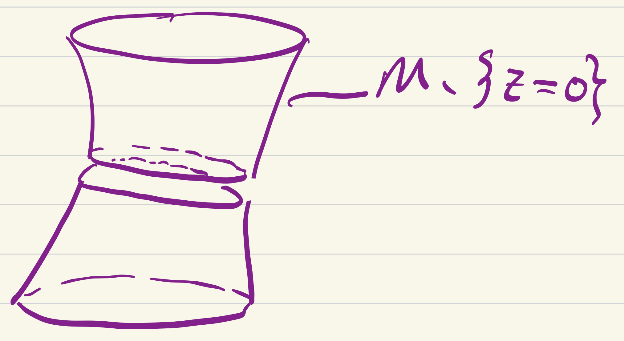
Ok, let’s hop right in! Say you have a $2$-manifold in ${\mathbb{R}}^3$ to start¹:

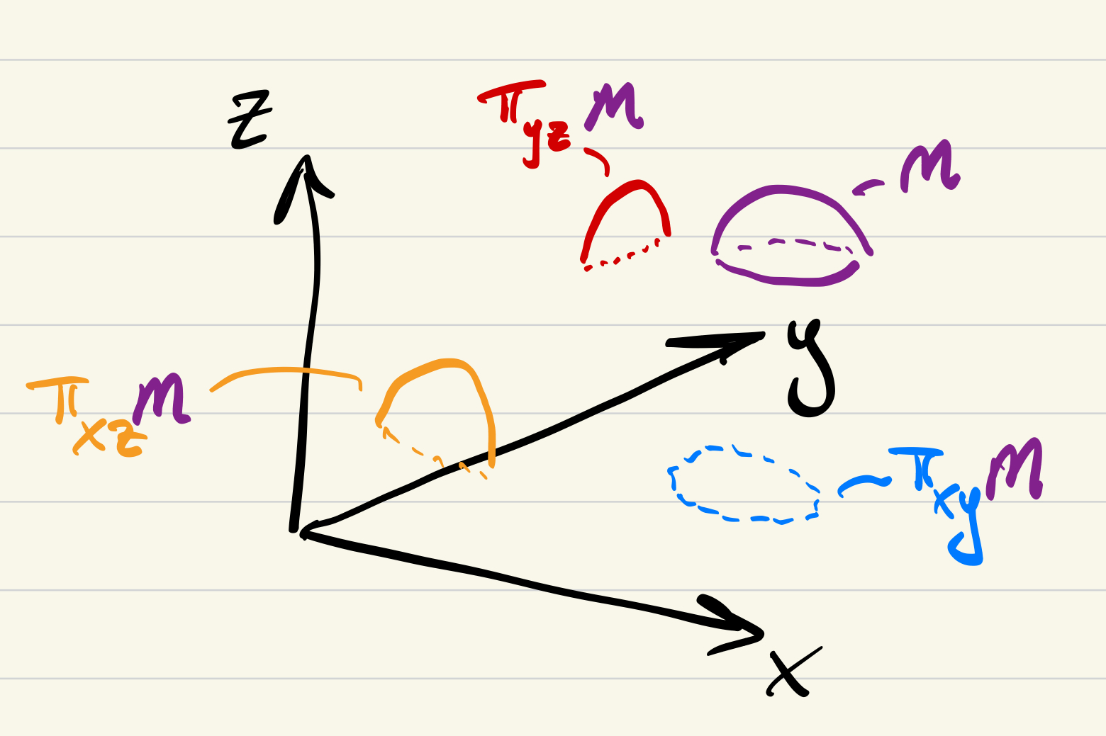
If we think of the purple manifold $M$ as being an open disk, representing a small neighborhood of some possibly larger 2-manifold, then we can see the projection onto the $xy$-plane is a diffeomorphism onto its image (an open disk in ${\mathbb{R}}^2$) while the projections onto the $yz$ and $xz$ planes are not open in ${\mathbb{R}}^2$! This is because the normal to $M$ is parallel to the $z$ axis inside $M$, (indeed, at the “top of the hill”) so the tangent plane at that point degenerates and projects to a line whenever we project onto a coordinate plane containing the $z$-direction.

For a more computational example, let’s try the hyperboloid $x^2+y^2-z^2=1$, and let’s see what happens near a few points.

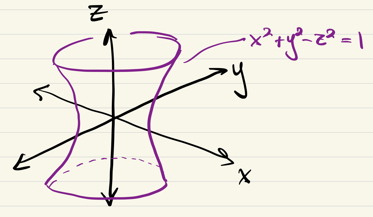
The tangent plane at a point is controlled by the jacobian of the defining equation, which for us is $⟨2x,2y,-2z⟩$.

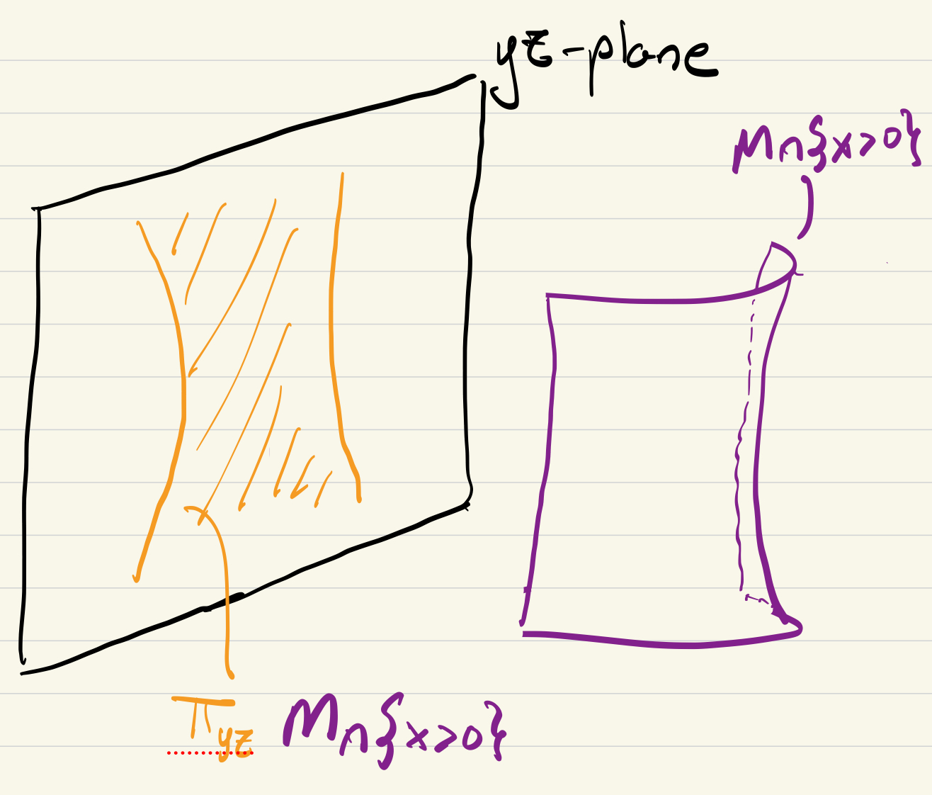
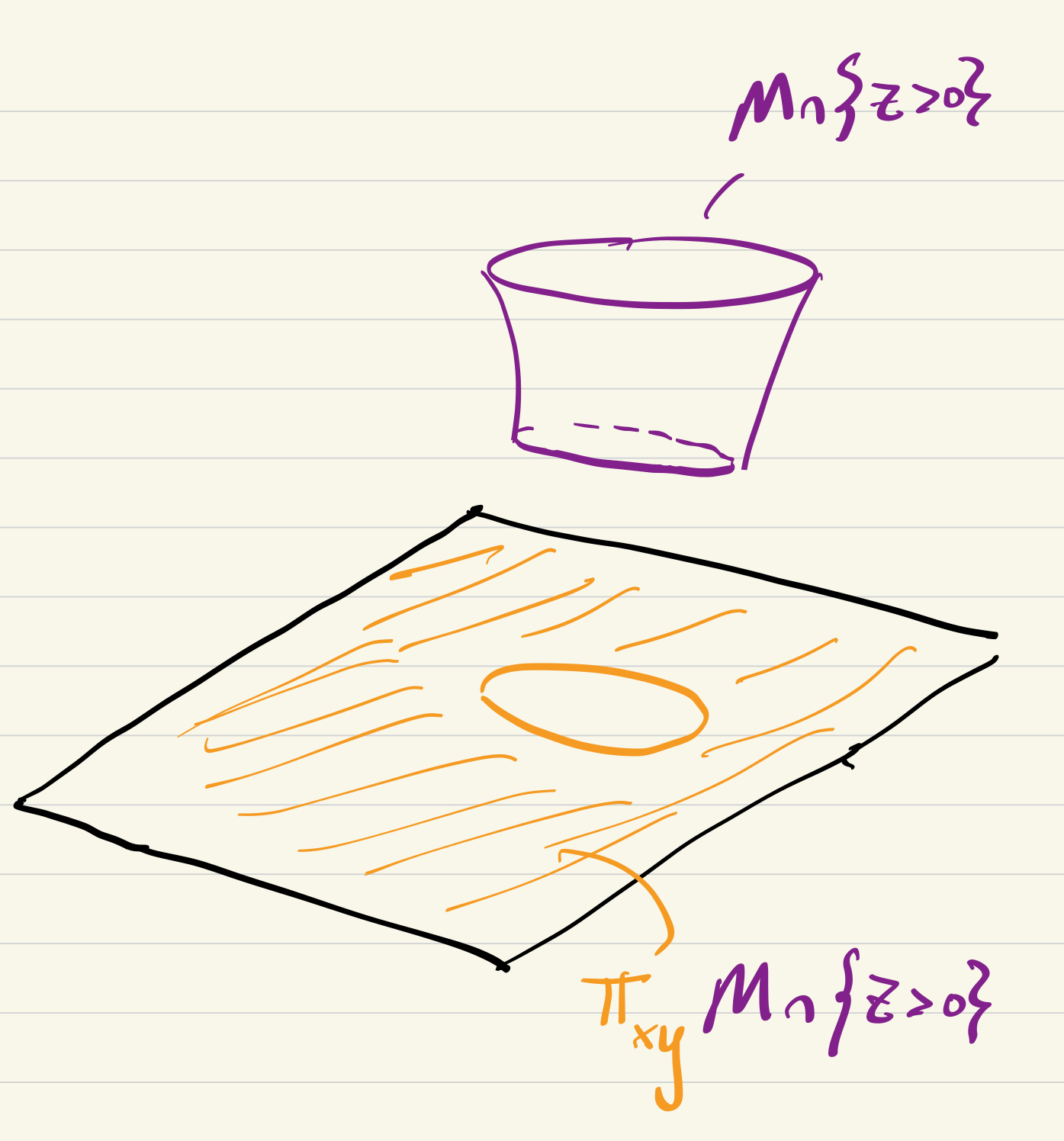
This gives us three (disconnected) charts: $\{2x\ne 0\}$, $\{2y\ne 0\}$, and $\{-2z\ne 0\}$, which we can see visually here (and we also drop the unnecessary scalars):

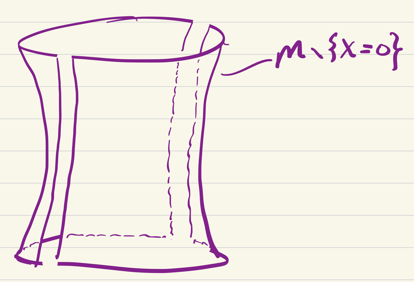
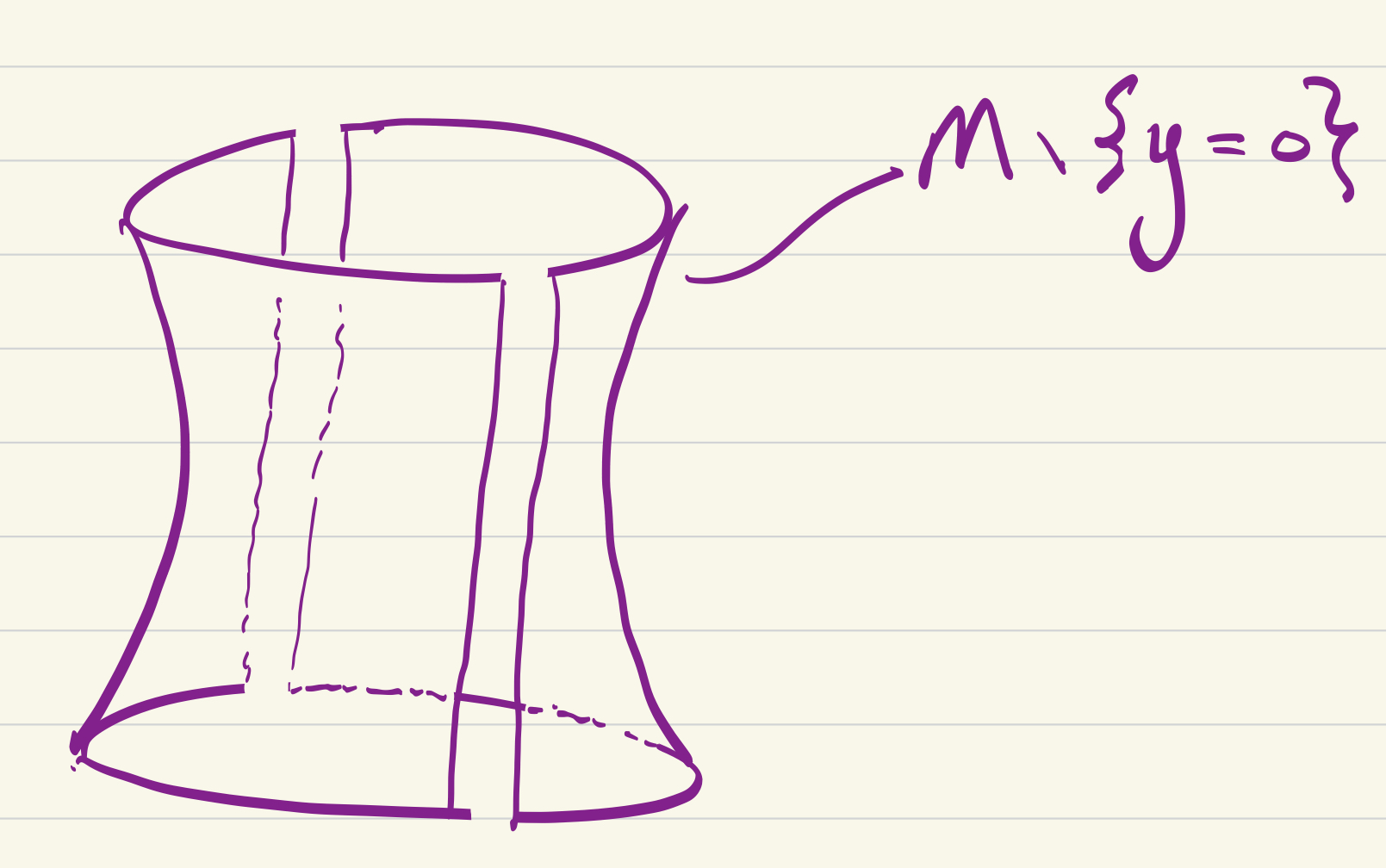
These turn into 6 honest-to-goodness charts where we turn the disconnected condition $\{x\ne 0\}$ into the pair of connected conditions $\{x>0\}$ and $\{x<0\}$. Indeed it’s easy to see that the 6 connected components in the above pictures are all diffeomorphic to an open subset of ${\mathbb{R}}^2$, and we can see this algebraically by projecting onto the plane avoiding the nonzero coordinate.

On $\{x>0\}$, for example, we have an open set of the $yz$-plane, shown here in orange:

Algebraically, we compute this chart by noting on $\{x>0\}$, we can solve for $x$ and (using the positive square root, since $x>0$) write our surface locally as

$$\{(+\sqrt{1+z^2-y^2},y,z)\mid z^2-y^2>-1\}$$

which is diffeomorphic in the obvious way to its projection onto the $yz$-plane

$$\{(y,z)\mid z^2-y^2>-1\}$$

so this is one of our charts!

Similarly, we can look at $\{z>0\}$, solve for $z$ and locally write our surface as

$$\{(x,y,+\sqrt{x^2+y^2-1})\mid x^2+y^2>1\}$$

which is diffeomorphic to $\{(x,y)\mid x^2+y^2>1\}$ – another chart.

On the intersection of these charts, $\{x,z>0\}$, it’s now easy to write down our transition maps (if one is so inclined):

Here our charts are the diffeomorphisms

$$\{(+\sqrt{1+z^2-y^2},y,z)\mid z^2-y^2>-1,z>0\}\to \{(y,z)\mid z^2-y^2>-1,z>0\}$$ $$\{(x,y,+\sqrt{x^2+y^2-1})\mid x^2+y^2>1,x>0\}\to \{(x,y)\mid x^2+y^2>1,x>0\}$$

so it’s easy to compose them to see our transition maps between these charts are

$$(y,z)\mapsto (+\sqrt{1+z^2-y^2},y):\{(y,z)\mid z^2-y^2>-1,z>0\}\to \{(x,y)\mid x^2+y^2>1,x>0\}$$ $$(x,y)\mapsto (y,+\sqrt{x^2+y^2-1}):\{(x,y)\mid x^2+y^2>1,x>0\}\to \{(y,z)\mid z^2-y^2>-1,z>0\}$$

---

For another example, let’s take a look at $S{L}_2(\mathbb{R})$, which is defined to be $\{\left(\begin{array}{cc}a& b\\ c& d\end{array}\right)\mid ad-bc=1\}\subseteq {\mathbb{R}}^4$.

Then the jacobian of our defining map is $⟨d,-c,-b,a⟩$, and we get charts corresponding to $\{d\ne 0\}$, $\{-c\ne 0\}$, $\{-b\ne 0\}$, and $\{a\ne 0\}$.

In the $\{d\ne 0\}$ chart, for instance, our defining equation looks like $a=\frac{1+bc}{d}$, so that $S{L}_2(\mathbb{R})$ looks locally like

$$\left\{\left(\begin{array}{cc}\frac{1+bc}{d}& b\\ c& d\end{array}\right)\right|d\ne 0\}{\cong }_{\text{diffeo}}\{(b,c,d)\in {\mathbb{R}}^3\mid d\ne 0\}$$

In the main post you can see how my friend Shane and I used this to compute the anchor map for a certain lie algebroid.

---

What about a codimension 2 example?

Let’s go back to our happy little hyperboloid, and intersect it with the surface $xyz=1$. That is, we want to consider the manifold

$$\{(x,y,z)|\begin{array}{c}{x}^2+y^2-z^2=1\\ xyz=1\end{array}\}$$

This is the levelset of the map ${\mathbb{R}}^3\to {\mathbb{R}}^2$ sending $(x,y,z)\mapsto (x^2+y^2-z^2,xyz)$ taking value $(1,1)$. So we compute the jacobian

$$\left(\begin{array}{ccc}2x& 2y& -2z\\ yz& xz& xy\end{array}\right)$$

and our charts are all the ways this matrix can have full rank. These conditions are:

• $2x\ne 0$ and $xz\ne 0$
• $2x\ne 0$ and $xy\ne 0$
• $2y\ne 0$ and $yz\ne 0$
• $2y\ne 0$ and $xy\ne 0$
• $-2z\ne 0$ and $yz\ne 0$
• $-2z\ne 0$ and $xz\ne 0$

If we look at the $\{2x\ne 0,xz\ne 0\}$ chart, we can ask sage to solve for $x$ and $z$ as functions of $y$:

So as in the previous hyperboloid example, we need to break this into four charts, depending on whether $x$ and $z$ are positive or negative.

Following the sage computation, in the $\{x>0,z>0\}$ chart, we can write our curve as

$$(\sqrt{\frac{1}{2}}\sqrt{-\frac{y^3-y-\sqrt{y^6-2y^4+y^2-4}}{y}},y,\frac{2\sqrt{\frac{1}{2}}}{y\sqrt{-\frac{y^3-y-\sqrt{y^6-2y^4+y^2-4}}{y}}})$$

which, by projecting out the $y$ coordinate, is diffeomorphic to the open subset of $\mathbb{R}$ where all these square roots are defined.

---

Ok, thanks for reading, all! This was extremely instructive for me, and hopefully it’s helpful to some of you as well! Sometimes it’s nice to just do some computations. Talk soon!

---