An Explicit Computation in Derived Algebraic Geometry

21 Jun 2025

Earlier this week my friend Shane and I took a day and just did a bunch of computations. In the morning we did some differential geometry, where he told me some things about what he’s doing with symplectic lie algebroids. We went to get lunch, and then in the afternoon we did some computations in derived algebraic geometry. I already wrote a blog post on the differential geometry, and now I want to write one on the derived stuff too!

I’m faaaaar from an expert in this stuff, and I’m sure there’s lots of connections I could make to other subjects, or interesting general theorem statements which have these computations as special cases… Unfortunately, I don’t know enough to do that, so I’ll have to come back some day and write more blog posts once I know more!

I’ve been interested in derived geometry for a long time now, and I’ve been sloooowly chipping away at the prerequisites – $\mathrm{\infty }$-categories and model categories, especially via dg-things, “classical” algebraic geometry (via schemes), and of course commutative and homological algebra. I’m lucky that a lot of these topics have also been useful in my thesis work on fukaya categories and TQFTs, which has made the time spent on them easy to justify!

I’ve just started reading a book which I hope will bring all these ideas together – Towards the Mathematics of Quantum Field Theory by Frédéric Paugam. It seems intense, but at least on paper I know a lot of the things he’s planning to talk about, and I’m hoping it makes good on its promise to apply its techniques to “numerous examples”. If it does, I’m sure it’ll help me understand things better so I can share them here ^_^.

In this post we’ll do two simple computations. In both cases we have a family of curves where something weird happens at a point, and in the “clasical” case this weirdness manifests as a discontinuity in some invariant. But by working with a derived version of the invariant we’ll see that at most points the classical story and the derived story agree, but at the weird point the derived story contains ~bonus information~ that renders the invariant continuous after all!

Ok, let’s actually see this in action!

---

First let’s look at what happens when we intersect two lines through the origin. This is the example given in Paugam’s book that made me start thinking about this stuff again.

Let’s intersect the $x$-axis (the line $y=0$) with the line $y=mx$ as we vary $m$. This amounts to looking at the schemes $\text{Spec}(k[x,y]/y)$ and $\text{Spec}(k[x,y]/y-mx)$. Their intersection is the pullback

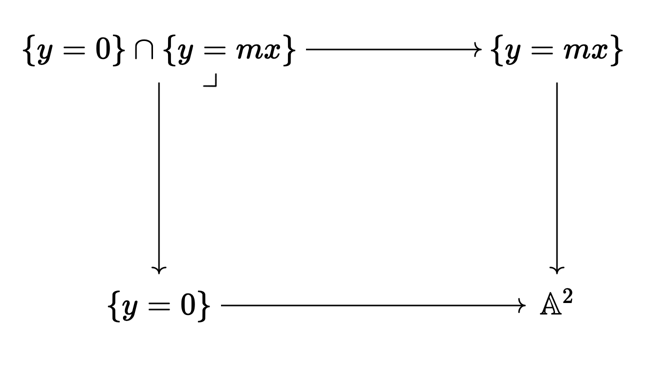
and so since everything in sight is affine, we can compute this pullback in $\text{Aff}={\text{CRing}}^{\text{op}}$ as a pushout in $\text{CRing}$:

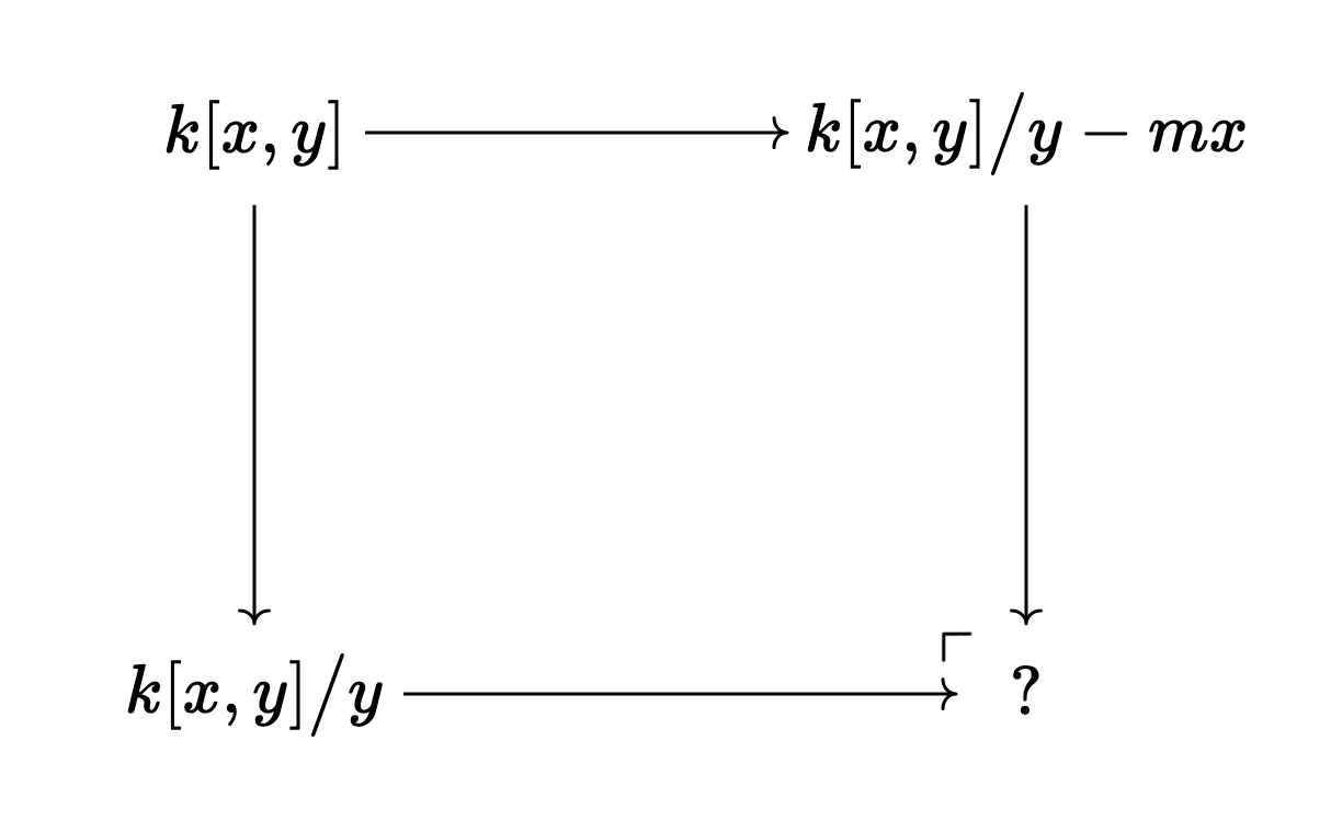
Pushouts in $\text{CRing}$ are given by (relative) tensor products, and so we compute

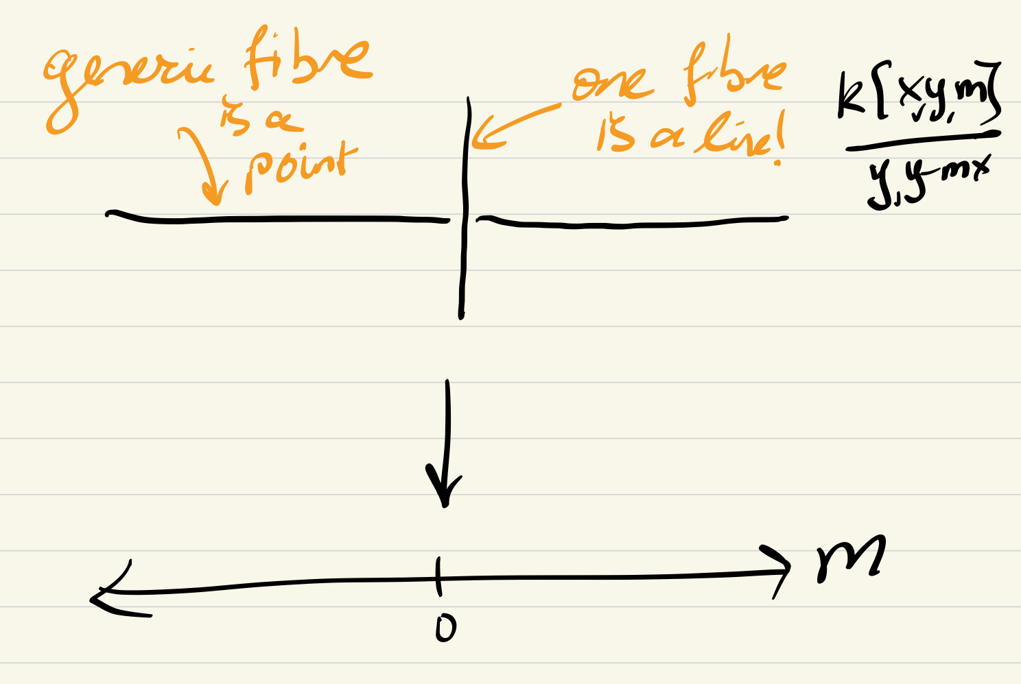
$$k[x,y]/(y){\otimes }_{k[x,y]}k[x,y]/(y-mx)\cong k[x,y]/(y,y-mx)\cong k[x]/(-mx)$$

which is $k$ when $m\ne 0$ and is $k[x]$ when $m=0$, so we’ve learned that:

• When $m\ne 0$ the intersection of $\{y=0\}$ and $\{y=mx\}$ is $\text{Spec}(k)$ – a single point¹.

• When $m=0$ the intersection is $\text{Spec}(k[x])$ – the whole $x$-axis.

This is, of course, not surprising at all! We didn’t really need any commutative algebra for this, since we can just look at it!

The fact that the dimension of the intersection jumps suddenly is related to the lack of flatness in the family of intersections $k[x,y,m]/(y,y-mx)\to k[m]$. Indeed, this doesn’t look like a very flat family!

We can also see it isn’t flat algebraically since tensoring with $k[x,y,m]/(y,y-mx)$ doesn’t preserve the exact sequence²

$$0\to k[m]\stackrel{-\cdot m}{⟶}k[m]⟶k\to 0$$

In the derived world, though, things are better. It’s my impression that here flatness is a condition guaranteeing the “naive” underived computation agrees with the “correct” derived computation. That is, flat modules $M$ are those for which $M{\otimes }^{\mathbb{L}}-$ and $M\otimes -$ agree for all modules $X$! I think that one of the benefits of the derived world is that we can pretend like “all families are flat”. I would love if someone who knows more about this could chime in, though, since I’m not confident enough to really stand by that.

In our particular example, though, this is definitely true! To see this we need to compute the derived tensor product of $k[x,y]/(y)$ and $k[x,y]/(y-mx)$ as $k[x,y]$-algebras. To do this we need to know the right notion of “projective resolution” (it’s probably better to say cofibrant replacement), and we can build these from (retracts of) semifree commutative dg algebras in much the same way we build projective resolutions from free things!

Here “semifree” means that our algebra is a free commutative graded algebra if we forget about the differential. Of course, “commutative” here is in the graded sense that $xy=(-1{)}^{\text{deg}(x)\text{deg}(y)}yx$.

For example, if we work over the base field $k$, then the free commutative graded algebra on $x_0$ (by which I mean an element $x$ living in degree $0$) is just the polynomial algebra $k[x]$ all concentrated in degree $0$. Formally, we have elements $1,x_0,x_0\otimes x_0,x_0\otimes x_0\otimes x_0,\dots$, and the degree of a tensor is the sum of the degrees of the things we’re tensoring, so that for $x_0$ the whole algebra ends up concentrated in degree $0$.

If we look at the free graded $k$-algebra on $x_1$, we again get an algebra generated by $x_1,x_1\otimes x_1,x_1\otimes x_1\otimes x_1,\dots$ except that now we have the anticommutativity relation $x_1\otimes x_1=(-1{)}^{1\cdot 1}{x}_1\otimes x_1$ so that $x_1\otimes x_1=0$. This means the free graded $k$-algebra on $x_1$ is just the algebra with $k$ in degree $0$, the vector space generated by $x$ in degree $1$, and the stipulation that $x^2=0$.

In general, elements in even degrees contribute symmetric algebras and elements in odd degrees contribute exterior algebras to the cga we’re freely generating.

What does this mean for our example? We want to compute the derived tensor product of $k[x,y]/y$ and $k[x,y]/y-mx$. As is typical in homological algebra, all we need to do is “resolve” one of our algebras and then take the usual tensor product of chain complexes. Here a resolution means we want a semifree cdga which is quasi-equivalent to the algebra we started with, and it’s easy to find one!

Consider the cdga $k[x,y,e]$ where $x,y$ live in degree $0$ and $e$ lives in degree $1$. The differential sends $de=y$, and must send everything else to $0$ by degree considerations (there’s nothing in degree $-1$). This cdga is semifree as a $k[x,y]$-algebra, since if you forget the differential it’s just the free graded $k[x,y]$ algebra on a degree 1 generator $e$!

So this corresponds to the chain complex

$$\cdots 0\to k[x,y]e\stackrel{d}{\to }k[x,y]\to 0$$

where $de=y$ is $k[x,y]$ linear so that more generally $d(pe)=p(de)=py$ for any polynomial $p\in k[x,y]$.

If we tensor this (over $k[x,y]$) with $k[x,y]/y-mx$ (concentrated in degree $0$) we get a new complex

$$\cdots 0\to (k[x,y]/y-mx)e\to (k[x,y]/y-mx)\to 0$$

where the interesting differential sends $pe\mapsto ey$ for any polynomial $p\in k[x,y]/y-mx$. Some simplification gives the complex

$$0\to k[x]\stackrel{-\cdot mx}{⟶}k[x]\to 0$$

whose homology is particularly easy to compute!

• $H_0=k[x]/mx$
• $H_1=\text{Ker}(mx)$

We note that $H_0$ recovers our previous computation, where when $m\ne 0$ we have $H_0=k$ is the coordinate ring of the origin³ and when $m=0$ we have $H_0=k[x]$ is the coordinate ring of the $x$-axis.

However, now there’s more information stored in $H_1$! In the generic case where $m\ne 0$, the differential $mx$ is injective so that $H_1$ vanishes, and our old “classical” computation saw everything there is to see. It’s not until we get to the singular case where $m=0$ that we see $H_1=\text{Ker}(mx)$ becomes the kernel of the $0$-map, which is all of $k[x]$!

The version of “dimension” for chain complexes which is invariant under quasi-isomorphism is the euler characteristic, and we see that now the euler characteristic is constantly $0$ for the whole family!

---

Next let’s look at some kind of “hidden smoothness” by examining the singular curve $y^2=x^3$. Just for fun, let’s look at another family of (affine) curves $y^2=x^3+tx$, which are smooth whenever $t\ne 0$. We’ll again show that in the derived world the singular fibre looks more like the smooth fibres.

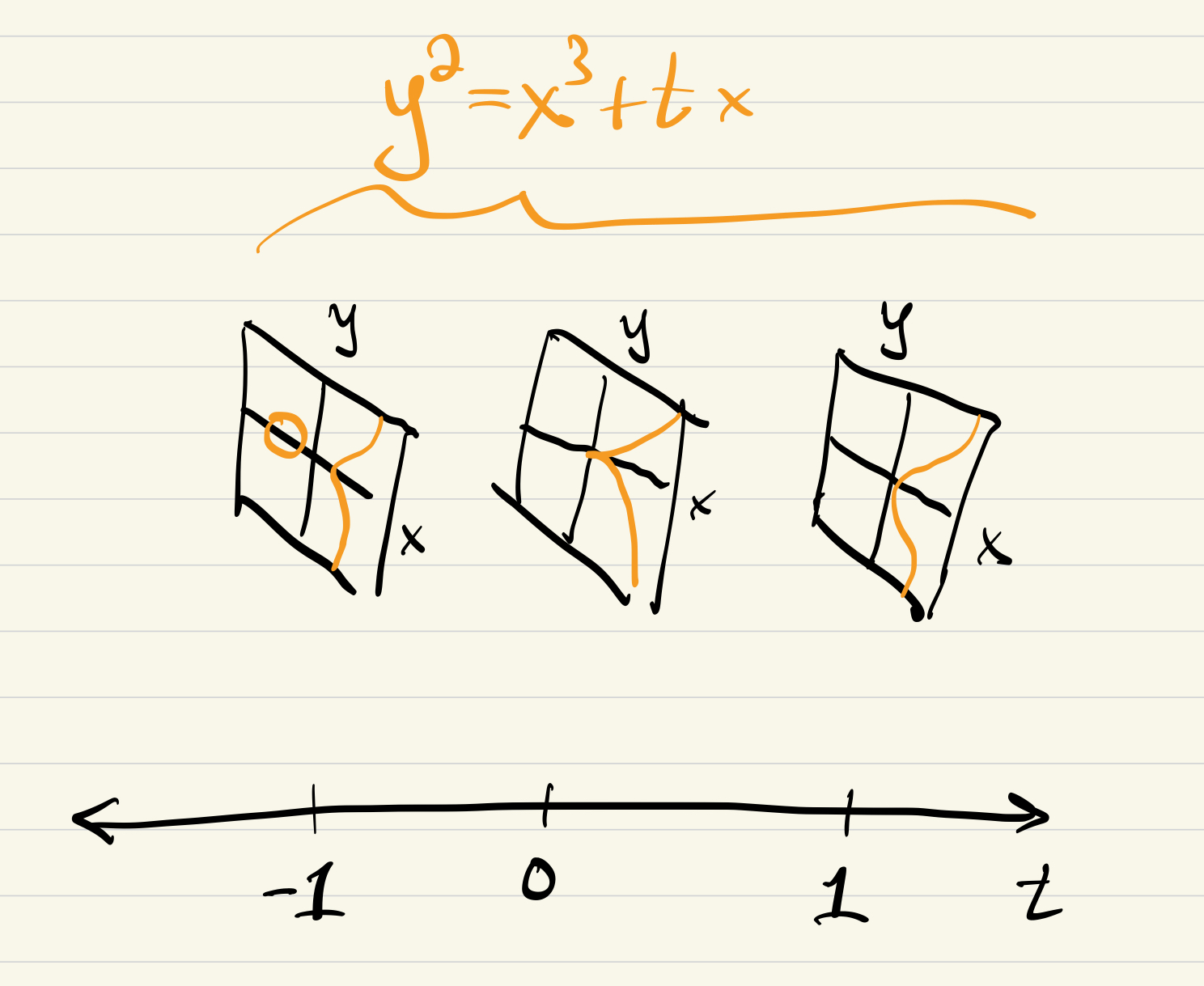
Smoothness away from the $t=0$ fibre is an easy computation, since we compute the jacobian of the defining equation $y^2-x^3-tx$ to be $⟨-3x^2-t,2y⟩$, and for $t\ne 0$ this is never $⟨0,0⟩$ for any point on our curve⁴ (We’ll work in characteristic 0 for safety). Of course, when $t=0$ $⟨-3x^2,2y⟩$ vanishes at origin, so that it has a singular point there.

To see the singularity, let’s compute the tangent space at $(0,0)$ for every curve in this family. We’ll do that by computing the space of maps from the “walking tangent vector” $\text{Spec}(k[ϵ]/{ϵ}^2)$ to our curve which deform the map from $\text{Spec}(k)$ to our curve representing our point of interest $(0,0)$.

Since everything is affine, we turn the arrows around and see we want to compute the space of algebra homs

$$k[x,y]/(y^2-x^3-tx)\to k[ϵ]/{ϵ}^2$$

so that the composition with the map $k[ϵ]/{ϵ}^2\to k$ sending $ϵ\mapsto 0$ becomes the map $k[x,y]/(y^2-x^3-tx)\to k$ sending $x$ and $y$ to $0$.

Since $k[x,y]/(y^2-x^3-tx)$ is a quotient of a free algebra, this is easy to do! We just consult the universal property, and we find a hom $k[x,y]/(y^2-x^3-tx)\to k[ϵ]/{ϵ}^2$ is just a choice of image $a+bϵ$ for $x$ and $c+dϵ$ for $y$, so that the equation $y^2-x^3-tx$ is “preserved” in the sense that $(c+dϵ{)}^2-(a+bϵ{)}^3-t(a+bϵ)$ is $0$ in $k[ϵ]/{ϵ}^2$.

Then the “deforming the origin” condition says that moreover when we set $ϵ=0$ our composite has to send $x$ and $y$ to $0$. Concretely that means we must choose $a=c=0$ in the above expression, so that finally:

The tangent space at the origin of $k[x,y]/(y^2-x^3-tx)$ is the space of pairs $(b,d)$ so that $(dϵ{)}^2-(bϵ{)}^3-t(bϵ)=0$ in $k[ϵ]/{ϵ}^2$. Of course, this condition holds if and only if $tb=0$, so that:

• When $t\ne 0$ the tangent space is the space of pairs $(b,d)$ with $b=0$, which is one dimensional.
• When $t=0$ the tangent space is the space of pairs $(b,d)$ with no further conditions, which is two dimensional!

Since we’re looking at curve, we expect the tangent space to be $1$-dimensional, and this is why we say there’s a singularity at the origin for the curve $y^2=x^3$….. But what happens in the derived world?

Now we want to compute the derived homspace. As before, a cofibrant replacement of our algebra is easy to find, it’s just $k[x,y,e]$ where $x$ and $y$ have degree $0$, $e$ has degree $1$ and and $de=y^2-x^3-tx$. Note that in our last example we were looking at quasifree $k[x,y]$-algebras, but now we just want $k$-algebras! So now this is the free graded $k$-algebra on 3 generators $x,y,e$, and our chain complex is:

$$0\to k[e]\stackrel{e\mapsto y^2-x^3-tx}{⟶}k[x,y]\to 0$$

We want to compute the derived ${\text{Hom}}^{\bullet }(-,-)$ from this algebra to $k[ϵ]/{ϵ}^2$, concentrated in degree $0$.

The degree $0$ maps are given by diagrams that don’t need to commute⁵!

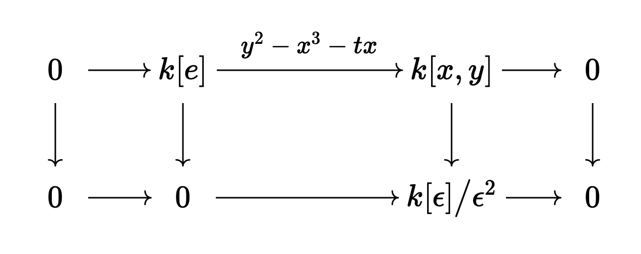
Of course, such maps are given by pairs $(a+bϵ,c+dϵ)$, which are the images of $x$ and $y$. As before, since we want the tangent space at $(0,0)$ we need to restrict to those pairs with $a=c=0$ so that ${\text{Hom}}^0(k[x,y]/y^2-x^3-tx,k[ϵ]/{ϵ}^2)=k^2$, generated by the pairs $(b,d)$.

Next we look at degree $-1$ maps, which are given by diagrams

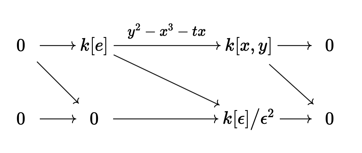
which are given by a pair $r+sϵ$, the image of $e$. Again, these need to restrict to the $0$ map when we set $ϵ=0$, so that $r=0$ and we compute ${\text{Hom}}^{-1}(k[x,y]/y^2-x^3-tx,k[ϵ]/{ϵ}^2)=k$, generated by $s$.

So our hom complex is

$$0\to \{(bϵ,dϵ)\}\to \{sϵ\}\to 0$$

where the interesting differential sends degree $0$ to degree $-1$ and is given by $df=d_{k[ϵ]/{ϵ}^2}\circ f-f\circ d_{k[x,y]/y^2-x^3-tx}$.

So if $f$ is the function sending $x\mapsto bϵ$ and $y\mapsto dϵ$ then we compute

$$(df)(e)=0\circ f-f(de)=-f(y^2-x^3-tx)=-tbϵ$$

So phrased purely in terms of vector spaces we see our hom complex is (living in degrees $0$ and $-1$):

$$0\to ⟨b,d⟩\stackrel{(-t0)}{⟶}⟨s⟩\to 0$$

So we compute

• $H^0=\text{Ker}((-t0))$
• $H^{-1}=⟨s⟩/\text{Im}((-t0))$

When $t\ne 0$, our map is full rank so that $H^0$ are the pairs $(b,d)$ with $b=0$ – agreeing with the classical computation. Then $H^{-1}=0$, so again we learn nothing new in the smooth fibres.

When $t=0$, however, our map is the $0$ map so that $H^0$ is the space of all pairs $(b,d)$ is two dimensional – again, agreeing with the classical computation! But now we see the $H^{-1}$ term, which is $1$ dimensional, spanned by $s$.

Again, in the derived world, we see the euler characteristic is constantly $1$ along the whole family!

There’s something a bit confusing here, since there seem to be two definitions of “homotopical smoothness”… On the one hand, in the noncommutative geometry literature, we say that a dga $A$ is “smooth” if it’s perfect as a bimodule over itself. On the other hand, though, I’ve also heard another notion of “homotopically smooth” where we say the cotangent complex is perfect. I guess it’s possible (likely?) that these should be closely related by some kind of HKR Theorem, but I don’t know the details.

Anyways, I’m confused because we just computed that the curve $y^2=x^3$ has a perfect tangent complex, which naively would make me think its cotangent complex is also perfect. But this shouldn’t be the case, since I also remember reading that a classical scheme is smooth in the sense of noncommutative geometry if and only if it’s smooth classically, which $y^2=x^3$ obviously isn’t!

Now that I’ve written these paragarphs and thought harder about things, I think I was too quick to move between perfectness of the tangent complex and perfectness of the cotangent complex, but I should probably compute the cotangent complex and the bimodule resolution to be sure…

---

Unfortunately, that will have to wait for another day! I’ve spent probably too many hours over the last few days writing this and my other posts on lie algebroids. I have some kind of annoying hall algebra computations that are calling my name, and I have an idea about a new family of model categories which might be of interest… But checking that something is a model category is usually hard, so I’ve been dragging my feet a little bit.

Plus, I need to start packing soon! I’m going to europe for a bunch of conferences in a row! First a noncommutative geometry summer school hosted by the institute formerly known as MSRI, then CT of course, and lastly a cute representation theory conference in Bonn.

I’m sure I’ll learn a bunch of stuff I’ll want to talk about, so we’ll chat soon ^_^. Take care, all!

---