Measure Theory and Differentiation (Part 2)

31 Aug 2021 - Tags: measure-theory-and-differentiation , analysis-qual-prep

This post has been sitting in my drafts since Feb 22, and has been mostly done for a long time. But, with my upcoming analysis qual, I’ve finally been spurred into finishing it. My plan is to put up a new blog post every day this week, each going through some aspect of the analysis that’s going to be on the qual. Selfishly, this will be great for my own preparation (I definitely learn through teaching) but hopefully this will also help future students who want to see a motivated treatment of the standard analysis curriculum.

The first half of this post is available here, as well as at the measure theory and differentiation tag. I’m also going to make a new tag for this series of analysis qual prep posts, and I’ll retroactively add part 1 to that tag.

With that out of the way, let’s get to the content!

In part 1 we talked about two ways of associating (regular, borel) measures to functions on $\mathbb{R}$:

To an increasing, right continuous $F$ we associate the measure $\mu_F$ defined by $\mu_F((a,b]) \triangleq F(b) - F(a)$. In the special case where $F$ is the identity function, we get Lebesgue Measure $m$ from this construction.
To a positive, locally $L^1$ function $f$ we associate the measure $m_f$ defined by $m_f(E) \triangleq \int_E f\ dm$.

Perhaps surprisingly, we can go the other way too!

Given a measure $\lambda$, we can define an increasing, right continuous function $F_\lambda$ so that $\mu_{F_\lambda} = \lambda$
Given a measure $\lambda \ll m$, we can find a function $f_\lambda$ so that $m_{f_\lambda} = \lambda$

These facts together give us a correspondence

\[\bigg \{ \text{increasing, right-continuous functions $F$} \bigg \} \longleftrightarrow \bigg \{ \text{regular borel measures $\mu_F$} \bigg \}\]

$\bigg \{ \text{positive locally $L^1$ functions $f$} \bigg \} \longleftrightarrow \bigg \{ \text{regular borel measures $m_f \ll m$} \bigg \}$

You should think of the increasing, right-continuous functions $F$ as being antiderivatives of the positive locally $L^1$ functions $f$, and theorems like the Lebesgue Differentiation Theorem link the (measure theoretic) Radon-Nikodym Derivative of $\mu_F$ with the classical derivative of $F$.

As an exercise to recap what we did in the last post, prove that every monotone function $F : \mathbb{R} \to \mathbb{R}$ is differentiable almost everywhere¹.

This result can be proven without the machinery of measure theory (see, for instance, Botsko’s An Elementary Proof of Lebesgue’s Differentiation Theorem), but the proof is much more delicate, and certainly less conceptually obvious. Also, some sort of machinery seems to be required. See here, for instance.

This should feel somewhat restrictive, though. There’s more to life than increasing, right continuous functions, and it would be a shame if all this machinery were limited to functions of such a specific form. Can we push these techniques further, and ideally get something that works for a large class of functions? Moreover, can we use these techniques to prove interesting theorems about this class of functions? Obviously I wouldn’t be writing this post if the answer were “no”, so let’s see how to proceed!

Differentiation is a nice motivation, but integration is theoretically much simpler. We can’t expect to be able to differentiate most functions, but it is reasonable to want to integrate them. With this in mind, rather than trying to guess the class of functions we’ll be able to differentiate, let’s try to guess the class of functions we’ll be able to integrate. Then we can work backwards to figure out what we can differentiate.

Previously we were restricting ourselves to positive locally $L^1$ functions. Since we want to meaningfully integrate our new class, it seems unwise to try and lift the $L^1$ condition. Positivity, however, seems like a natural thing to drop. Let’s be optimistic and see what happens if we work with all (complex valued) $L^1$ functions!

The correspondence says to take $f$ and send it to the measure $m_f(E) \triangleq \int_E f \ dm$. Of course, now that $f$ is complex valued, this integral might take complex values as well! To that end, let’s introduce the idea of Complex Valued Measures and see how much of measure theory we’re able to recover.

If we meditate on what properties $m_f$ will have, we land on the following definition²:

A Complex Measure on a $\sigma$-algebra $\mathcal{A}$ is a function $\nu : \mathcal{A} \to \mathbb{C}$ so that

$\nu \ \emptyset = 0$
$\nu \left ( \bigcup E_n \right ) = \sum \nu E_n$ for any disjoint $E_n$. Importantly, this sum automatically converges absolutely³.

Notice $\nu E$ is never allowed to be $\infty$! This is an important difference between complex and positive measures⁴.

⚠ Be careful! Now that our measures allow nonpositive values, we might “accidentally” have $\nu E = 0$. If $E$ is the disjoint union of $E_+$ and $E_-$, where $\nu E_+ = 3$ and $\nu E_- = -3$ (say), then $\nu E = 0$, even though we really shouldn’t call it a nullset!

Because of this, we redefine the notion of nullset to be more restrictive: We say $E$ is $\nu$-null if and only if $\nu A = 0$ for every $A \subseteq E$.

As an exercise, can you come up with a concrete signed measure $\nu$ for which $\nu E = 0$ even though $E$ is not null?

As another exercise, why does this agree with our original definition of nullsets when we restrict to positive measures?

Now, we could try to build measure theory entirely from scratch in this setting. But it seems like a waste, since we’ve already done so much measure theory already… It would be nice if there were a way to relate signed measures to ordinary (unsigned) measures and leverage our previous results!

We know that $m_{f+g} = m_f + m_g$ in the unsigned case. So in the complex case, it’s natural to try and get this linearity to go further! But we know we can write any complex function $f : X \to \mathbb{C}$ as a linear combination of $4$ positive functions, by breaking up into real and imaginary parts, then positive and negative parts:

\[f = (f_R^+ - f_R^-) + i (f_I^+ - f_I^-)\]

So we should expect

\[m_f = m_{f_R^+} - m_{f_R^-} + i (m_{f_I^+} - m_{f_I^-})\]

and the Jordan Decomposition Theorem says⁵ that we can decompose every complex measure $\nu$ in exactly this way!

Formally, it says that every complex measure $\nu$ decomposes uniquely into a linear combination of finite positive measures $\nu = (\nu_R^+ - \nu_R^-) + i (\nu_I^+ - \nu_I^-)$ with the bonus property that $\nu_R^+ \perp \nu_R^-$ and $\nu_I^+ \perp \nu_I^-$. Here, as usual, $\perp$ means that two measures are mutually singular, which we should intuitively think of as having disjoint support.

It can still be nice to work with an unsigned measure directly sometimes, rather than having to split our measure into $4$ parts. Thankfully we have a convenient way of doing so!

There is a positive measure $|\nu|$, called the Total Variation of $\nu$, which is defined so that

\[|m_f| = m_{|f|}.\]

This possesses all the amenities the notation suggests, including:

(Triangle Inequality) $\lvert \nu + \mu \rvert \leq \lvert \nu \rvert + \lvert \mu \rvert$
(Operator Inequality) $\lvert \nu E \rvert \leq \lvert \nu \rvert E$
(Continuity) $\nu \ll \lvert \nu \rvert$

In fact, the collection of complex measures on $X$ assembles into a Banach Space under the norm $\lVert \nu \rVert \triangleq \lvert \nu \rvert X$.

Ok. This has been a lot of information. How do we actually compute with a complex measure? Thankfully, the answer is easy: We use the Jordan Decomposition. We define

\[\int f \ d\nu \triangleq \left ( \int f \ d\nu^+_R - \int f \ d\nu^-_R \right ) + i \left ( \int f \ d\nu^+_I - \int f \ d\nu^-_I \right ).\]

In particular, in order to make sense of this integral, we need to know that $f$ is in $L^1$ for each of these measures. So again, we just define

\[L^1(\nu) \triangleq L^1(\nu^+_R) \cap L^1(\nu^-_R) \cap L^1(\nu^+_I) \cap L^1(\nu^-_I).\]

As an easy exercise, show that the dominated convergence theorem is true when we’re integrating against $\nu$!

We can split up $\nu$ if we need to, but oftentimes we don’t. Remember that if $\nu = m_f$ (which is the whole reason we embarked on this journey!) we should have $\int g \ d\nu = \int gf \ dm$.

Show using the definition of $\int g \ d\nu$ that we gave that $\int g \ dm_f = \int gf \ dm$ actually holds.

So, as a quick example computation:

\[\int_0^{2\pi} x^2 \ dm_{e^{ix}} = \int_0^{2\pi} x^2 e^{ix} dm = 4 \pi - 4 I \pi^2\]

Notice, as usual, that once we’ve phrased the integral in terms of $dm$, we can simply use integration by parts, or any other tricks we know (such as asking sage) to compute the integral.

Now, that example might have felt overly simplistic. After all, it was mainly a matter of moving the $e^{ix}$ from downstairs below the $m$ to upstairs inside the integral. What if we needed to integrate against a more complicated complex measure? Thankfully, up to singular measures, every measure is of this simple form!

Remember last time, we had a structure theorem that told us every measure is of the form $m_f$, possibly plus a “singular” part $\lambda$. Moreover, the function $f$ so that $\nu = m_f + \lambda$ was the “derivative” of $\nu$, and this led us to the fruitful connection between measure theoretic and classical derivatives. Thankfully, the same theorem is still true in the complex setting!

Lebesgue-Radon-Nikodym Theorem

If $\nu$ is a $\sigma$-finite signed measure and $\mu$ is a $\sigma$-finite positive measure⁶, then $\nu$ decomposes uniquely as

\[\nu = \lambda + \mu_f\]

for a $\sigma$-finite measure $\lambda \perp \mu$ and $\mu_f(E) \triangleq \int_E f\ d\mu$.

As in the unsigned case, we write $f = \frac{d\nu}{d\mu}$.

I realized while writing this post that last time I forgot to mention an important aspect of the Radon-Nikodym derivative! It satisfies the obvious laws you would expect a “derivative” to satisfy⁷. For instance:

(Linearity) $\frac{d(a\nu_1 + b\nu_2)}{d\mu} = a\frac{d\nu_1}{d\mu} + b\frac{d\nu_2}{d\mu}$
(Chain Rule) If $\nu \ll \mu \ll \lambda$, then $\frac{d \nu}{d\lambda} = \frac{d \nu}{d\mu} \frac{d\mu}{d\lambda}$

It’s worth proving each of these. The second is harder than the first, but it’s not too bad.

At last, we have a complex measure theoretic notion of “derivative”, as well as half of the correspondence we’re trying to generalize:

Given an $L^1$ function $f : \mathbb{R} \to \mathbb{C}$ we can build a (complex) measure $m_f$, and given a complex measure $m_f \ll m$, we can recover $f$ as the derivative $\frac{d m_f}{dm}$.

But which functions will generalize the increasing right continuous ones? The answer is Functions of Bounded Variation!

To see why bounded variation functions are the right things to look at, let’s remember how the correspondence went in the unsigned case: We took an unsigned measure $\mu$ and looked at (up to sign of $x$) the (increasing, right continuous) function $F_\mu(x) = \mu \left ( (0,x] \right )$.

Now, for a complex measure $\nu$, we know we can write it as a combination of unsigned functions, $\nu = (\nu_R^+ - \nu_R^-) + i (\nu_I^+ - \nu_I^-)$. So what would happen if we just… did our old construction to each of these individually, then put them back together?

Then if we look at the real part, we would be looking at functions $F_{\nu_R^+} - F_{\nu_R^-}$, where each $F_{\nu_R^\pm}$ is increasing and right continuous. Moreover, since complex measures are finite, we know that each of these functions is bounded as well. We could define bounded variation functions as exactly this class! That is, $f$ is bounded variation if and only if its real and imaginary parts are both a difference of bounded increasing functions!

Of course, nothing in life is so simple, and for what I assume are historical reasons, this is not the definition you’re likely to see (despite it being equivalent).

The more common definition of bounded variation is slightly technical, and is best looked up in a reference like Folland. The idea, though, is that $F$’s ability to wiggle should be bounded – whence the name⁸.

For instance, $F(x) = x^2\sin \left ( \frac{1}{x} \right )$ is bounded variation, while $G(x) = x^2 \sin \left ( \frac{1}{x^2} \right )$ is not. A picture is worth a thousand words, and indeed $F$ has a maximum rate of wiggle:

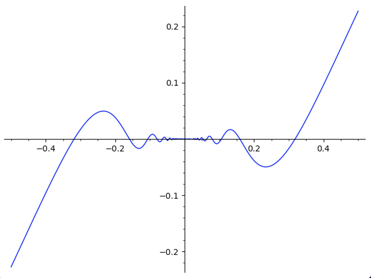
Even though $F$ wiggles faster and faster as $x \to 0$, the vertical distance it travels gets small fast enough to compensate. Contrast that with $G$:

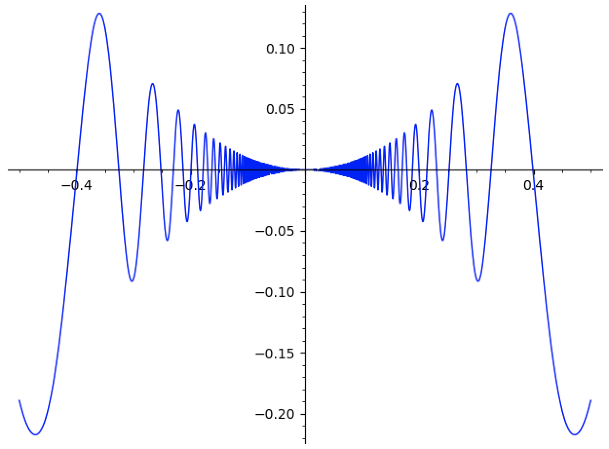
whose wiggle-density is obviously less controlled⁹.

We also get some results that will be familiar from the last post. These are akin to the properties of monotone functions that relate them to increasing right continuous functions, and thus measures.

If $F$ is bounded variation, then it has at most countably many discontinuities
If $F$ is bounded variation, then it can be made right continuous by looking at $F^+(x) \triangleq \lim_{y \to x} F(y)$. By (1) these are equal almost everywhere.

Lastly, if $F$ is bounded variation, then $\displaystyle \lim_{x \to - \infty} F(x)$ exists and is finite. We say $F$ is Normalized if $\displaystyle \lim_{x \to -\infty} F(x) = 0$. We can always normalize $F$ by replacing it with $\displaystyle F^N = F - \lim_{x \to -\infty} F(x)$. Notice $F$ and $F^N$ have the same derivative (since they differ by a constant).

This brings us to our punchline!

If $\nu$ is a complex borel measure on $\mathbb{R}$, then

\[F_\nu(x) \triangleq \nu \left ( (-\infty, x] \right )\]

is normalized bounded variation.

Conversely, if $F$ is normalized bounded variation, then there exists a unique complex borel measure $\nu_F$ so that $F = F_{\nu_F}$.

So we have correspondences:

\[\bigg \{ \text{normalized bounded variation functions $F$} \bigg \} \longleftrightarrow \bigg \{ \text{regular complex borel measures $\nu_F$} \bigg \}\]

$\bigg \{ \text{$L^1$ functions $f$} \bigg \} \longleftrightarrow \bigg \{ \text{regular complex borel measures $m_f \ll m$} \bigg \}$

Here, $F_{m_f}$ is the antiderivative of $f$, and each $F$ is differentiable with $F’ = \frac{d \nu_F}{dm}$ almost everywhere. Moreover, $F’$ is $L^1$, and if $\nu_F \ll m$ we have $F(x) = \int_{-\infty}^x F’$.

In fact, the class of functions $F$ so that $\nu_F \ll m$ is the largest class of functions making the fundamental theorem of calculus true¹⁰:

Lebesgue Fundamental Theorem of Calculus

The Following Are Equivalent for a function $F : [a,b] \to \mathbb{C}$:

$F$ is differentiable almost everywhere on $[a,b]$, $F’$ is in $L^1([a,b])$, and $F(x) - F(a) = \int_a^x F’ \ dm$
$F(x) - F(a) = \int_a^x f \ dm$ for some $f \in L^1([a,b])$
$F$ is bounded variation and $\nu_F \ll m$ on $[a,b]$.

As one last exercise for the road, you should use this machinery to prove Rademacher’s Theorem:

If $F : \mathbb{R} \to \mathbb{C}$ is locally lipschitz, then $F$ is differentiable almost everywhere¹¹.

The idea is to show that $F$ is basically increasing and right continuous, then apply the results from the part $1$ of this blog post. We can get increasing-ness by possibly replacing $F$ by $-F$. We can get right continuity by replacing $F$ with $F^+(x) = \lim_{y \to x^+} F(y)$, and checking that $F = F^+$ almost everywhere. ↩
It’s easy to wonder what complex measures are good for. One justification is the one we’re giving in this post: they provide a clean way of extending the fundamental theorem of calculus to a broader class of functions.

There’s actually much more to say, though. Complex measures are linear functionals, where we take a function $f$ and send it to the number $\int f\ d\nu$. One version of the Riesz Representation Theorem says that every linear functional on $C_0 X$ is of this form (when $X$ is locally compact, hausdorff).

This is great, because it means we can bring measure theory to bear on problems in pure functional analysis. As one quick corollary, this lets us transfer the dominated convergence theorem to the setting of functionals. Of course, without the knowledge of complex measures, we wouldn’t be able to talk about this, since most functionals are complex valued!

At this point, the category theorist in me needs to mention a cute result from Emily Riehl’s Category Theory in Context. There are two functors $\mathsf{cHaus} \to \mathsf{Ban}$ (that is, from compact hausdorff spaces with continuous maps to (real) banach spaces with bounded linear maps). The first sends $X$ to its banach space of signed measures, and the second sends $X$ to the (real) dual of its continuous functions $X \mapsto CX^*$. It turns out these functors are naturally isomorphic (see also Hartig’s The Riesz Representation Theorem Revisited).

It seems reasonable to me that there would also be a natural isomorphism between the complex dual of the functions vanishing at infinity and the space of compelx valued measures, but I can’t find a reference and I’m feeling too lazy to work it out myself right now… Maybe one day a kind reader will leave a comment letting me know? ↩
By the Riemann Rearrangement Theorem. ↩
In fact, since $\nu$ can never be infinite, we will focus our attention on functions $f$ which are $L^1$, rather than just locally $L^1$ as we were able to do before. If $f$ is real valued, then we can relax this a little bit by using signed measures, but I won’t be going into that in this post. ↩
Really it’s a statement about real valued signed measures, and so it allows for either $\pm \infty$ (but not both!) to occur. We won’t need this extra flexibility, though.

I went back and forth for a long time on whether to include a discussion about signed measures in this post. Eventually, I decided it made the post too long, and it encouraged me to include details that obscure the main points. I want these posts to show the forest rather than the trees, and here we are. ↩
Notice for us $\mu$ will almost always be lebesgue measure. The theorem is true much more broadly, though, and we might ask “why do we care about more general measures?”. The answer is that there are other measures which are also easy to compute in practice (haar measures, and counting measures on countable sets come to mind).

With this generality, we can know for sure that we can work in any space which admits an effectively computable ($\sigma$-finite) measure (and there are lots of such spaces besides $\mathbb{R}^n$).

Any space with a computable notion of integration also admits a computable notion of integrating complex measures by application of Radon-Nikodym! ↩
If you’re familiar with product measures, there’s actually a useful fact:

If $\nu_1 \ll \mu_1$ and $\nu_2 \ll \mu_2$ and everything in sight is $\sigma$-finite, then we have $\nu_1 \times \nu_2 \ll \mu_1 \times \mu_2$, and
\[\frac{d(\nu_1 \times \nu_2)}{d(\mu_1 \times \mu_2)}(x_1, x_2) = \frac{d \nu_1}{d \mu_1}(x_1) \frac{d \nu_2}{d \mu_2}(x_2)\]
This is great, since it means to integrate against some product measure on $\mathbb{R}^2$, we can separately integrate against each component. ↩
Mathematicians like to use words like “variation” and “oscillation” rather than “wiggliness”. I can’t imagine why. ↩
Another way of viewing the issue (particularly in light of the upcoming theorem) is that $G’$ is not $L^1$. It turns out that a $C^1$ function is bounded variation if and only if its derivative is $L^1$. That is, if and only if $\int \lvert G’ \rvert \lt \infty$. ↩
There is actually a characterization of $\nu_F \ll m$ that doesn’t refer to $\nu_F$. If $F$ satisfies this condition, then $F$ is called absolutely continuous. Thankfully, any $F$ which satisfies this is automatically bounded variation. ↩
For this, it might be useful to look up the more technical definitions of “bounded variation” and “absolutely continuous” that I’ve omitted in this post. Both cam be found in Chapter $3.6$ of Folland’s Real Analysis: Modern Techniques and their Applications. ↩