Life in Johnstone's Topological Topos 1 -- Fundamentals
03 Jul 2024 - Tags: life-in-the-topological-topos , featured , topos-theory
I’ve been thinking a lot about the internal logic of topoi again, and I want to have more examples of topoi that I understand well enough to externalize some statements. There’s more to life than just a localic $\mathsf{Sh}(B)$, and since I’m starting to feel like I understand that example pretty well, it’s time to push myself to understand other important examples too!
In particular, it would be nice to throw some gros topoi into the mix, and where better to start than Johnstone’s topological topos? This topos is fairly small (which makes explicit computation easy) and is very well studied (which makes finding references and examples merely annoying instead of totally impossible). Eventually I’ll want to learn about the effective topos1 (and other realizability topoi more generally), various smooth topoi, etc. but let’s take them on one-at-a-time!
The topological topos $\mathcal{T}$ is a world where every set is intrinsically a space. What does this mean?
Well, if we’re working in $\mathsf{Set}$, then a space is a set $X$ equipped with some ~bonus structure~. This structure can take a lot of forms, but one ubiquitous example is that of a topology $\tau \subseteq \mathcal{P}(X)$.
Then if you want to work with spaces, you have to constantly keep track of what topology you’re working with. For example, there’s lots of topologies you can put on $X \times Y$, and we need to make sure we choose the right one to act like the product of the spaces $(X,\tau)$ and $(Y,\sigma)$.
Nowadays the “right” topology is usually “obvious2”, but this is only because we’re able to stand on the shoulders of countless 20th century mathematicians! I think most people would be hard-pressed to come up with, say, the compact-open topology if they hadn’t seen it before!
Of course, carrying around this ~bonus structure~ becomes most pronounced when working with continuous maps! Now, instead of just defining a function and moving on with your life, we’re constantly burdened to check that our function $X \to Y$ actually respects the topologies involved! Otherwise it isn’t a continuous function $(X,\tau) \to (Y, \sigma)$! There are some friends of mine who are constantly complaining that algebraic topologists never check that things are continuous, and honestly I’m sympathetic. But it can be a real hassle to check these things all the time…
Thankfully there’s a better way!
Every set in $\mathcal{T}$ is, by its very nature, a space! There’s no need to choose the “right” topology, or to check that your function is “continuous”. Inside $\mathcal{T}$, it’s literally impossible to write down a function that isn’t continuous, because there’s no ~bonus structure~ to respect! This is what we mean when we say the topology is intrinsic.
This is great for a couple reasons. First, say you build a type $X$ in Martin-Löf Type Theory (MLTT). We know how to interpret MLTT in any topos, so by interpreting $X$ in $\mathcal{T}$ we learn that our type $X$ is automatically a space! Understanding this relationship between types and topology has been a staple in many people’s careers, but I want to single out Martín Escardó as someone whose papers I’ve been reading lately (and who I talk to fairly often on mastodon). These conversations were a big part of the reason I decided to spend some time trying to understand $\mathcal{T}$.
Second, by the same logic, any theorem we’re able to prove constructively is automatically true in $\mathcal{T}$. That is, any constructive theorem is automatically true “continuously”, giving us a theorem for topological structures! Of course, in order to use these theorems, we need to understand how objects inside the topological topos $\mathcal{T}$ relate to honest topological spaces in “the real world”3.
In the process of learning about $\mathcal{T}$, I had to work out a bunch of examples, which I’d love to share! Even though all of this is probably “well known to experts”, I found a lot of it pretty hard to find, so hopefully this blog post is still useful for people ^_^.
Let’s get started!
What Is $\mathcal{T}$?
First, what even is the topological topos? It’s sheaves on some site, of course, but which one?
Write \(\mathbb{N}_\infty\) for the one point compactification of $\mathbb{N}$. This is the space \(\{0,1,2,3,\ldots,\infty\}\) topologized so that a convergent sequence $(x_n) \to x_\infty$ in $X$ is exactly a continuous map $\mathbb{N}_\infty \to X$4.
Then let’s look at the full subcategory of $\mathsf{Top}$ spanned by \(\{1, \mathbb{N}_\infty \}\). This becomes a site if we give it the canonical topology $J$, and we define the topological topos $\mathcal{T}$ to be sheaves on this site.
We’ll say more about this definition in a minute, but first let’s see how we can picture objects of $\mathcal{T}$.
A presheaf on this site is a pair of sets $X(1)$ and $X(\mathbb{N}_\infty)$ with a bunch of maps connecting them:
- There’s a map \(n^* : X(\mathbb{N}_\infty) \to X(1)\) for each $n$, plus a map \(\infty^* : X(\mathbb{N}_\infty) \to X(1)\)
- There’s a unique map \(!^* : X(1) \to X(\mathbb{N}_\infty)\)
- For every continuous function \(f : \mathbb{N}_\infty \to \mathbb{N}_\infty\) there’s a map \(f^* : X(\mathbb{N}_\infty) \to X(\mathbb{N}_\infty)\).
You should think of elements of $X(1)$ as the points of $X$, and the elements of \(X(\mathbb{N}_\infty)\) as (witnesses to) convergent sequences in $X(1)$. Indeed, if \(p \in X(\mathbb{N}_\infty)\), then we’ll write $p_n$ for \(n^*(p)\) (resp. $p_\infty$ for \(\infty^* p\)) and $p$ should be thought of as a witness or proof that the sequence $p_n$ converges to $p_\infty$ in $X(1)$5.
The unique map \(!^*\) sends a point $x \in X(1)$ to a distinguished proof that the constant $x$ sequence converges to $x$, and the functions \(f^*\) “reindex” a convergent sequence. So if $p$ is a proof that $x_n \to x_\infty$, then $f^* p$ is a proof that $x_{fn} \to x_{f \infty}$ too.
The sheaf condition for the canonical topology guarantees that if every subsequence of $x_n$ converges to $x_\infty$, the whole sequence $x_n$ converges to $x_\infty$ too6.
Can you prove that this is reasonable?
If \(x_n \to x\) in some topological space \(X\), and \(f : \mathbb{N}_\infty \to \mathbb{N}_\infty\) is continuous, why must \(x_{fn} \to x_{f \infty}\)?
You might find it helpful to case on whether \(f(\infty) = \infty\) or not.
As a cute exercise can you find a simple description of the arrows in $\mathcal{T}$? That is, for a natural transformation between two sheaves?
solution
A natural transformation between $X$ and $Y$ is a pair of functions $$f_1 : X(1) \to Y(1)$$ $$f_{\mathbb{N}_\infty} : X(\mathbb{N}_\infty) \to Y(\mathbb{N}_\infty)$$ So that whenever $p$ is a proof that $x_n \to x_\infty$, $f_{\mathbb{N}_\infty}(p)$ is a proof that $f_1(x_n) \to f_1(x_\infty)$. Moreover, $f_{\mathbb{N}_\infty}$ should respect the distinguished proofs that constant sequences converge (so $f_{\mathbb{N}_\infty}(!^* x) = !^* f_1(x)$) as well as reindexing (so $f_{\mathbb{N}_\infty}(g^* p) = g^* (f_{\mathbb{N}_\infty} p)$)Now every topological space $X$ gives an object $よX = \mathsf{Top}(-,X)$ in the topos7, where $よX(1) = X$ and \(よX(\mathbb{N}_\infty) = \{ \text{continuous functions } f : \mathbb{N}_\infty \to X \}\). That is, the underlying set of $よX$ is exactly the underlying set of $X$, and for every convergent sequence in $X$ there is a unique proof that that sequence converges (represented by the sequence itself).
If we restrict attention to the full subcategory of sequential spaces, then $よ$ is a fully faithful embedding into $\mathcal{T}$. This shouldn’t be too surprising, since the sequential spaces are exactly those spaces whose topologies are determined by a knowledge of which sequences converge!
Importantly, you should think of this is a super mild condition, since lots of natural spaces of interest are sequential. Just to name a few:
- all metric spaces
- more generally, all first countable spaces
- every CW-complex
- every noetherian ring spectrum
This tells us that a huge subcategory of topological spaces embeds fully faithfully into $\mathcal{T}$! Later we’ll say more about how computations in $\mathcal{T}$ translate to computations in the real world, but this is a good first indication that they should be closely related!
There’s another definition of $\mathcal{T}$ which you’re also likely to see.
Having $X(1)$ around explicitly as a set of points is helpful for exposition and intuition, but it turns out to not change the topos if we work without it! Intuitively, we can recover the points from the constant maps \(n : \mathbb{N}_\infty \to \mathbb{N}_\infty\).
With this in mind, some authors define $\mathcal{T}$ to be the sheaves on just the full subcategory of $\mathsf{Top}$ spanned by \(\{ \mathbb{N}_\infty \}\). That is, they define it to be sheaves on the monoid of continuous endomorphisms of \(\mathbb{N}_\infty\). See, for instance, The Elephant (A2.1.11(j)).
This gives a different informal justification for the close connection between $\mathcal{T}$ and sequential spaces. Indeed, objects of a sheaf topos can be thought of as being glued together from objects of the underlying site. In case you’re working with a presheaf topos, we take all the ways to glue things together, but in general a grothendieck topology forces us to restrict attention to those gluings which are “nice” in some sense.
So, with this smaller site in hand, one way to think about objects in $\mathcal{T}$ is as copies of \(\mathbb{N}_\infty\) that are “glued together nicely”. And one can show that the sequential spaces are exactly the quotients of disjoint unions of copies of \(\mathbb{N}_\infty\)! This also tells us that, in some sense, the other objects of $\mathcal{T}$ are just copies of \(\mathbb{N}_\infty\) glued together in more exotic ways, for instance by gluing two copies of \(\mathbb{N}_\infty\) literally on top of each other to get multiple witnesses to the convergence of the same sequence!
But how do we know that these two definitions agree? I wasn’t able to find this written down anywhere, but it’s easy to check for ourselves!
The key observation is that \(\{ \mathbb{N}_\infty \}\) is a dense subsite of \(\{ \mathbb{N}_\infty, 1 \}\). Here I’m using set-builder notation to mean a full subcategory of $\mathsf{Top}$ equipped with the canonical topology.
$\ulcorner$ Indeed, to check this, we only need to show that every object in \(\{ \mathbb{N}_\infty, 1 \}\) is covered by maps with domain in \(\{ \mathbb{N}_\infty \}\). But the identity function \(\mathbb{N}_\infty \to \mathbb{N}_\infty\) covers, and the unique map \(\mathbb{N}_\infty \to 1\) covers too.
Since \(\{ \mathbb{N}_\infty \}\) is a full subcategory of \(\{ \mathbb{N}_\infty, 1 \}\), the second condition of the comparison lemma is trivial, and we learn that the geometric map induced by the inclusion is an equivalence.
In particular, the two common definitions really do give equivalent topoi! $\lrcorner$
So, finally, what is the Canonical Topology?
For the site with two objects, \(\{1, \mathbb{N}_\infty\}\), every (nonempty) family of arrows \(\{X_\alpha \to 1 \}\) is covering. So the interesting question is what a covering family of \(\mathbb{N}_\infty\) looks like.
If $S$ is an infinite subset of $\mathbb{N}$, we write $f_S$ for the unique monotone map \(\mathbb{N}_\infty \to \mathbb{N}_\infty\) whose image is \(S \cup \{ \infty \}\).
A family \(\{X_\alpha \to \mathbb{N}_\infty\}\) is covering if and only if both
- It contains every constant map \(1 \to \mathbb{N}_\infty\)
- For every infinite $T \subseteq \mathbb{N}$, there is a further infinite subset $S \subseteq T$ with \(f_S : \mathbb{N}_\infty \to \mathbb{N}_\infty\) in the family
In particular, if a family contains every constant map \(1 \to \mathbb{N}_\infty\) and a “tail of an infinite sequence” \(f_{\{x \geq N\}}\) for some $N$, then that family is covering.
So, roughly, to prove that something “merely exists” in $\mathcal{T}$, we have to provide a witness for every finite $n$, and these witnesses should converge to the witness for $\infty$.
If we want to use the site with one object \(\{ \mathbb{N}_\infty \}\), the condition is almost exactly the same. A family of maps is covering if and only if both
- every constant map \(\mathbb{N}_\infty \to \mathbb{N}_\infty\) is in the family
- For each infinite $T \subseteq \mathbb{N}$, there’s a further infinite $S \subseteq T$ so that $f_S$ is in the family.
This, unsurprisingly, doesn’t make too much difference. But note that the site with two objects is obviously local in the sense of The Elephant (C3.6.3(d)). So we learn that the global sections functor $\Gamma : \mathcal{T} \to \mathsf{Set}$ which takes an object $X$ to its set of points $X(1)$ admits the usual left adjoint characteristic of geometric morphisms (giving a set $X$ the discrete topology) but also a further right adjoint (giving a set $X$ the indiscrete topology).
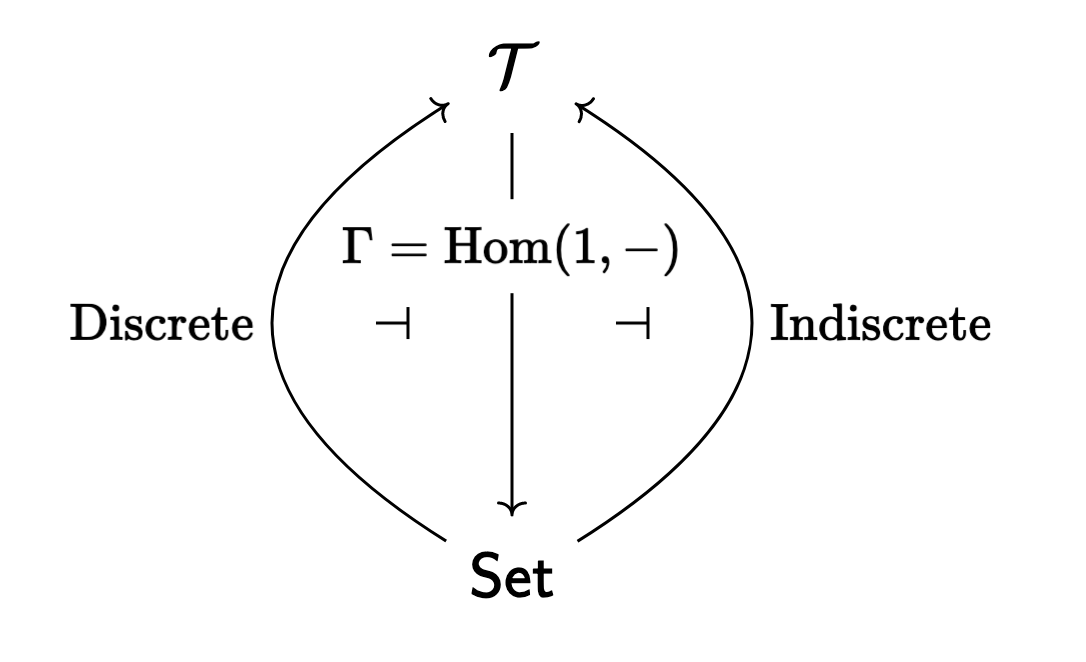
In the original paper, Johnstone moreoever shows that the essential point $\mathsf{Set} \to \mathcal{T}$ given by this indiscrete arrow is the unique global point of $\mathcal{T}$.
How Does $\mathcal{T}$ Relate to $\mathsf{Top}$?
Here’s the tl;dr for this section, for ease of reference.
We have a sequence of fully-faithful embeddings of bicartesian closed categories, each of which admits a left adjoint, as shown below:
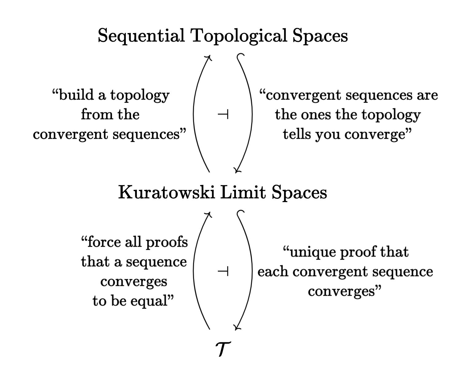
The embeddings preserve all limits (as right adjoints) but moreover preserve the cartesian closed structure, as well as certain “nice” colimits (in particular, all colimits involved in the creation of CW-complexes). The exact definition of “nice” here is explained in Johnstone’s original paper, but includes the coproduct. Additionally, the image of a map $X \to Y$ of sequential spaces (with $Y$ sequentially hausdorff) as computed in $\mathcal{T}$ is just the set theoretic image equipped with the quotient topology (Corollary 6.4 in the original paper).
The left adjoints preserve all colimits, and moreover preserve finite products (and thus, in particular, models of algebraic theories).
Lastly, in case we restrict to the full subcategory of “sequentially hausdorff spaces”, in the sense that every convergent sequence has a unique limit, then the adjunction $\text{Seq} \leftrightarrows \text{Kur}$ is an adjoint equivalence!
Here $\text{Seq}$ is bicartesian closed, $\text{Kur}$ is locally cartesian closed, $\mathcal{T}$ is a topos, and the embeddings preserve all of this structure. Thus one can say that at each level we add new “type constructors”, as shown in the following diagram (stolen from Martín Escardó):
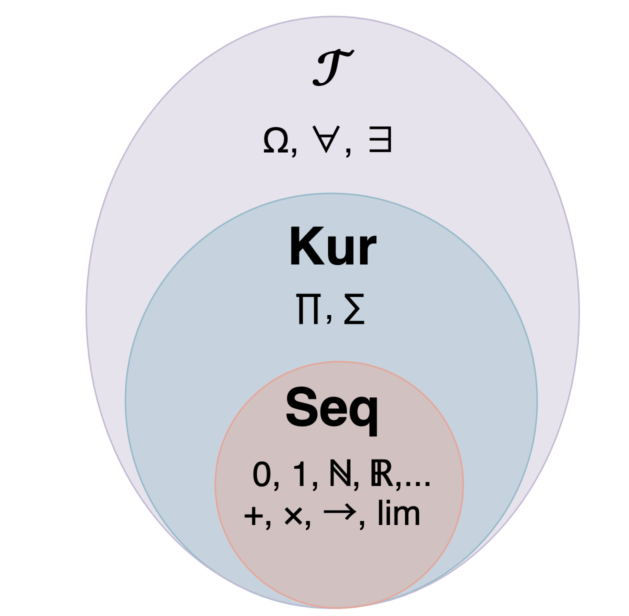
Colimits in $\text{Seq}$ are computed as in $\mathsf{Top}$, so in particular the “nice colimits” that get preserved between $\text{Seq}$ and $\mathcal{T}$ agree with colimits in $\mathsf{Top}$.
The relationship of limits in $\text{Seq}$ to limits in $\mathsf{Top}$ is more subtle. If you only care about (quotients of) second countable spaces, then the bicartesian closed structure on $\text{Seq}$ (and thus in $\mathcal{T}$) agrees with the usual bicartesian closed structure on the “convenient category” of compactly generated spaces. In particular, function spaces get the compact-open topology.
If your spaces are locally compact, then the (finite) product in $\text{Seq}$ (and thus in $\mathcal{T}$) agrees with the product in $\mathsf{Top}$.
That’s a lot, so let’s go more in depth into what all of this means, haha.
We’ll start with the definition of a Kuratowski Limit Space (also called a subsequential space):
A Kuratowski Limit Space is a set $X$ equipped with a set of Convergent Sequences in $X$ subject to the following axioms:
- For every $x \in X$, the constant sequence $(x)$ converges to $x$
- If $(x_n)$ converges to $x$, then every subsequence of $(x_n)$ converges to $x$ too
- If, for some $x$, every subsequence of $(x_n)$ contains a further subsequence converging to $x$, then the whole sequence $(x_n)$ already converges to $x$.
We moreover call $X$ Sequentially Hausdorff if it satisfies the bonus axiom
- If $(x_n)$ converges to $x$ and $(x_n)$ converges to $y$, then $x=y$.
A function $f : X \to Y$ between limit spaces is called continuous if whenever $x_n \to x$, we have $fx_n \to fx$.
Every sequential topological space is automatically a limit space, where we just let the convergent sequences be the (topologically) convergent sequences. Moreover, there’s a fully faithful embedding of limit spaces into $\mathcal{T}$ where we let $X(1) = X$ and \(X(\mathbb{N}_\infty)\) be the set of convergent sequences in $X$.
As a (not so tricky) exercise, you might want to verify that this map from $\mathsf{Kur}$ to presheaves is actually always a sheaf.
This basically amounts to comparing axiom (3) for limit spaces to the definition of a cover of \(\mathbb{N}_\infty\).
Taken together, we have fully faithful embeddings
\[\mathsf{Seq} \hookrightarrow \mathsf{Kur} \hookrightarrow \mathcal{T}\]In fact, Johnstone’s original paper shows that $\mathsf{Kur}$ is the quasitopos of $\lnot \lnot$-separated sheaves in $\mathcal{T}$! Thus the embedding $\mathsf{Kur} \hookrightarrow \mathcal{T}$ admits a finite product preserving left adjoint, and the locally cartesian closed structure of $\mathsf{Kur}$ agrees with that of $\mathcal{T}$ (see A1.5.9 in the elephant).
Concretely, this left adjoint takes an object of $\mathcal{T}$ and fogets how a sequence converges, only remembering that it converges! Said another way, it identifies any proofs $p$ and $q$ with $p_n = q_n$ for all \(n \in \mathbb{N}_\infty\).
Moreover, the embedding $\mathsf{Seq} \hookrightarrow \mathsf{Kur}$ also admits a finite product preserving left adjoint!
We say a subset $U \subseteq X$ is Sequentially Open if whenever \(x_n \to a \in U\), some tail of $x_n$ is entirely contained in $U$. It’s easy to see that the set of sequential open subsets forms a topology on $X$, and indeed our reflector sends a limit space \((X,\{\text{convergent sequences}\})\) to the sequential space \((X,\{\text{sequential opens}\})\). This functor moreover preserves finite products8, which is Proposition 3.1 in Menni and Simpson’s Topological and limit-space subcategories of countably-based equilogical spaces9.
Also, notice that this reflection possibly adds new convergent sequences. Maybe our limit space $X$ knows about some convergent sequences, but once we actually build a topology to make these sequences converge in the usual sense, there might accidentally be more convergent sequences than we started with!
Conversely, the subobjects of a space $X \in \mathcal{T}$ come from taking a subset of the points and a subset of the convergent sequences. So we see this is exactly what the kuratowski limit spaces are! They’re the subobjects of sequential spaces, where we may have forgotten about certain sequences that “would converge” if we still had our open sets.
In general, we can think of objects in $\mathsf{Seq}$ as honest spaces, with points and all the convergent sequences that should exist. Objects in $\mathsf{Kur}$ are almost honest spaces, we just might have forgotten about a few convergent sequences that “should” be there if we remembered the whole topology. But there’s still only “one way” for any given sequence to converge. Objects in $\mathcal{T}$ are like spaces which might have forgotten some convergent sequences, and which have ~bonus data~ attached to them giving multiple inequivalent proofs that these sequences converge!
But this intuitive picture tells us how to get an honest space from your favorite object $X \in \mathcal{T}$! We take $X(1)$ as our set of points, and a subset of $X(1)$ is open exactly when it’s sequentially open, forgetting the data of the multiple proofs of convergence.
The fact that the reflectors preserve finite products tells us that the $\mathsf{Seq}$ and $\mathsf{Kur}$ are exponential ideals in $\mathcal{T}$. Thus they’re both cartesian closed, and the embeddings preserve the cartesian closed structure! It’s not hard to see the embeddings $\mathsf{Seq} \hookrightarrow \mathsf{Kur}$ and $\mathsf{Kur} \hookrightarrow \mathcal{T}$ preserve coproducts, so that we get the promised embeddings of bicartesian closed categories.
Lastly, the cartesian closed structure on $\mathsf{Seq}$ is the one you would expect from viewing it as a “convenient category of spaces”. The exponential is (usually) the compact-open topology! You can read more about the subtleties in Escardó, Lawson, and Simpson’s Comparing Cartesian closed categories of (core) compactly generated spaces, but the gist is that you get the compact-open topology whenever you’re working with (quotients of) second countable spaces!
From this information, there’s a few simple corollaries that I want to mention explicitly, since they give more relationships between $\mathsf{Top}$, $\mathsf{Seq}$, and $\mathcal{T}$.
First, fully faithful functors reflect isomorphisms, so if we can prove in $\mathcal{T}$ that two spaces are isomorphic, it means they must be isomorphic in $\mathsf{Seq}$ too. But then all functors preserve isomorphisms, so that we get an isomorphism in $\mathsf{Top}$ too! Thus, we can show two sequential spaces are homeomorphic by working entirely in $\mathcal{T}$! The converse argument (using the fully faithful embedding $\mathsf{Seq} \hookrightarrow \mathsf{Top}$) shows that two homeomorphic sequential spaces are also isomorphic in $\mathcal{T}$, so that we can detect every homeomorphism just by working in $\mathcal{T}$.
Similarly, if $A$ and $B$ are both sequential, then a map $A \to B$ is monic in $\mathsf{Top}$, if and only if it’s monic in $\mathsf{Seq}$ if and only if it’s monic in $\mathcal{T}$! In all cases, the monics are exactly the continuous injections10. This tells us that anything we “expect” to be a subobject in $\mathcal{T}$ actually is. But note that in $\mathsf{Top}$ we might have nonsequential subspaces of a sequential space (any non-frechet sequential space will do. see here) and similarly in $\mathcal{T}$ we might have nonsequential subspaces of a sequential space (indeed, every kuratowski limit space is a subobject in $\mathcal{T}$ of a sequential space). Nonetheless, open/closed subspaces of a sequential space will be sequential in both $\mathsf{Top}$ and in $\mathcal{T}$.
Dually, if $A \to B$ is an epi in $\mathcal{T}$, then it’s an epi in $\mathsf{Seq}$, and thus an epi in $\mathsf{Top}$ (since the inclusion $\mathsf{Seq} \to \mathsf{Top}$ is a left adjoint, and preserves epis). But there’s no reason to suspect an epi in $\mathsf{Top}$ to remain an epi in $\mathcal{T}$.
This is great and all, but the only way to really get some intuition for how computations in $\mathcal{T}$ relate to computations in $\mathsf{Top}$ is to actually do some computation and check! So let’s do that! Let’s start with a few important types representing various kinds of proposition. These will be important for building new types later, and for understanding how to externalize them.
$2$
This is the discrete space with two points \(\{\top,\bot\}\). This is sequential (every finite space is, and so is every discrete space), so behaves exactly as you would expect. Note that the convergent sequences are all eventually constant!
We think of $2$ as the space of Decidable Propositions, so that maps $X \to 2$ classify decidable properties of $X$. These are the same as clopen subsets of $X$, and thus might be quite rare. Notice that, in $\mathcal{T}$, $2$ doesn’t form a complete lattice! It has finite joins and meets, of course, and we can can build the continuous functions $\land, \lor : 2 \times 2 \to 2$ quite easily. Thinking of $2$ as classifying clopen subobjects, this corresponds to the fact that a finite union/intersection of clopen sets is clopen. Indeed, if $A,B \subset X$ are clopen, classified by maps $\chi_A, \chi_B : X \to 2$, then the map $\lambda (x:X). \chi_A(x) \land \chi_B(x) \ : X \to 2$ classifies exactly $A \cap B$.
This tells us immediately that $2$ cannot have countable joins/meets. We can see this via continuity, since the map $\bigwedge : 2^\mathbb{N} \to 2$ with \(\bigwedge \alpha = \begin{cases} \top & \forall n . \alpha(n) = \top \\ \bot & \text{otherwise} \end{cases}\) is not continuous! (and neither is $\bigvee$. In both cases, do you see why?)
We can instead see this by thinking of $2$ as classifying clopen subsets, since if $\bigwedge$ or $\bigvee$ existed, we could use them with classfiying maps to show the countable intersection/union of clopen sets is clopen. But of course we know this is false!
As a last aside, it’s not hard to see that $2$ being countably complete corresponds exactly to the Weak Limited Principle of Omniscience (WLPO), so that this shows $\mathcal{T} \not \models \text{WLPO}$. We’ll talk more about omniscience principles in part 3, but it’s nice to mention.
$\Sigma$
This is the sierpinski space, which also has two points \(\{\top,\bot\}\), but with the topology \(\{\emptyset, \{\top\}, \Sigma \}\). This is sequential (every finite space is), where every sequence converges to $\bot$ and the sequences converging to $\top$ are only the eventually constantly $\top$ ones.
We think of $\Sigma$ as the space of Open Propositions, since maps $X \to \Sigma$ classify the open subspaces of $X$. By the same logic as before, it’s easy to show that $\Sigma$ is a lattice with finite meets and joins (indeed, we can build the maps $\lor$ and $\land$ using the yoneda lemma in $\mathsf{Seq}$ knowing that open subspaces are closed under finite unions and intersections).
A similar yoneda argument shows that $\Sigma$ is a complete lattice, since homs into $\Sigma$ are open subspaces, and arbitrary unions of opens are open, so these operations must be represented by joins $\bigvee$ on $\Sigma$. But it’s kind of fun to show directly that $\bigvee : \Sigma^\mathbb{N} \to \Sigma$ is continuous (and more generally so is $\bigvee : \Sigma^\kappa \to \Sigma$ for any cardinal $\kappa$).
As a cute aside, this tells us that $\Sigma$ must be closed under arbitrary meets as well… But of course, the arbitrary intersection of open subspaces isn’t open. Do you see what’s going on there?
$\Sigma^c$
This is the “co-sierpinski space”. It has two points \(\{\top, \bot\}\) but the topology is \(\{\emptyset, \{\bot\}, \Sigma^c\}\). Again it’s sequential, but now we see that every sequence converges to $\top$, while only the eventually constant $\bot$ sequences converge to $\bot$.
Unsurprisingly, this is the space of Closed Propositions, and maps into $\Sigma^c$ classify closed subspaces of $X$. The same logic as before shows $\Sigma^c$ is a complete lattice, but now we have direct access to $\bigwedge$, since closed subspaces are closed under arbitrary intersection!
$\nabla 2 = \Omega_{\lnot \lnot}$
At this point you know what’s going on. This space has two points, \(\{\top, \bot\}\) with the indiscrete topology (the only opens are $\emptyset$ and $\nabla 2$), so here every sequence coverges to both $\top$ and $\bot$. We think of this as the space of all “classical” propositions, since a map $X \to \nabla 2$ is exactly the same thing as a “classical” subspace of $X$. That is, a subset of the points equipped with the induced topology.
This interpretation also makes it more believable that it should correspond to $\Omega_{\lnot \lnot}$, the double-negation closed propositions, as this does represent the “classical” propositions, where we really care about subsets of points (which are complemented, so satisfy LEM), and then take whatever topology makes the universal propety work (which happens to be the subspace topology).
Notice that this is again a complete lattice. We can see this either because $\nabla 2$ is indiscrete, so every function into it is continuous (in particular, the arbitrary join/meet functions are continuous), or by using yoneda again (since arbitrary unions/intersection of subsets of points are again subsets of points).
$\Omega$
This is the subobject classifier, or the space of all propositions! Maps $X \to \Omega$ classify all subspaces, even the possibly nonclassical ones. That is, this is the first time we’re able to build a limit space, rather than an “honest” sequential space!
Notice that, for $2$ (resp. for $\Sigma$, $\Sigma^c$, and $\nabla 2$) if we start with a sequential space $X$ and a decidable (resp. open or closed or classical) proposition $\varphi : X \to 2$ (resp. $\Sigma$, $\Sigma^c$, $\nabla 2$), then the pullback
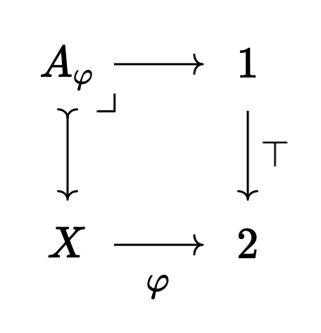
exists in $\mathsf{Seq}$, and is an honest clopen (resp. open, closed, classical) subspace of $X$.
Note that this $A_\varphi$ is an object above $X$, so if we want to access it in the type theory we have to compose with the map from $X \to 1$. That is, in the type theory $A_\varphi$ (the subspace classified by $\varphi$) is represented by $\Sigma_{x:X} \varphi$, as we would expect.
Now, what does the space of all propositions look like in $\mathcal{T}$? Well, we know that $2$, $\Sigma$, $\Sigma^c$, and $\nabla 2$ are all sequential spaces. So there’s a unique convergence proof for each sequence. It turns out the ability to “remember” only some convergent sequences (which puts is into the world of kuratowski limit spaces) can be coded up by more interesting proofs of convergence! Let’s see how!
Johnstone shows that $\Omega$ has two points $\top$ and $\bot$, and for any sequence $x_n$ of $\top$s and $\bot$s
- there’s exactly one proof that $x_n \to \bot$
- there’s one proof that $x_n \to \top$ for each “closed ideal of subsets of $\mathbb{N}$” whose “extent” is \(\{n \mid x_n = \top \}\).
Here a “closed ideal of subsets of $\mathbb{N}$” is a pair $(E,I)$ where $E \subseteq \mathbb{N}$ is called the extent of the closed ideal of subsets.
In the above, $I$ is a family of infinite subsets of $E$, so that
- if $S$ is an infinite subset of $T$ and $T \in I$, then $S \in I$ too
- if every infinite subset of $T$ has a further infinite subset in $I$, then $T \in I$ too.
These correspond, basically, to axioms (2) and (3) for limit spaces. This will make sense once we understand how this subobject classifier actually classifies subobjects!
Say that we have a subobject $A \hookrightarrow X$. That is, we remember only some of the points of $X$, and we only remember some of the (proofs of) convergent sequences. This had better be classified by a unique map (read: natural transformation) $\ulcorner A \urcorner : X \to \Omega$.
On points, we have \(\ulcorner A \urcorner(x) = \begin{cases} \top & x \in A \\ \bot & x \not \in A \end{cases}\), but what do we do for a proof $p$ that $x_n \to x_\infty$?
Well, to what extent is $(x_n) \in A$? Each point of the sequence is either in $A$ or isn’t, so a sequence $x_n$ in $X$ produces a sequence of $\top$s and $\bot$s given by $\omega_n = \ulcorner A \urcorner(x_n)$.
If $x_\infty \not \in A$ (that is, if $\omega_\infty = \bot$), then life is easy. We send $p$ to the unique proof that $\omega_n \to \bot$. If instead $x_\infty \in A$, then there are lots of proofs that $\omega_n \to \top$, indexed by these closed ideals of subsets. So to decide where $p$ should go, we need a natural choice of $(E,I)$ associated to our sequence $x_n$.
We’ll let \(E = \{ n \mid x_n \in A \}\) be the extent to which $x_n \in A$. Next, we have to say which infinite subsets of $E$ live in $I$. Given any infinite subset $T \subseteq E$, we can restrict $x_n$ to a subsequence of indices in $T$. Since $E$ is exactly the indices where $x_n \in A$, this restriction $x_n \upharpoonright T$ is a sequence in $A$. Now we say that $T \in I$ if and only if the restriction $p \upharpoonright T$ proving that $x_n \upharpoonright T \to x_\infty$ in $X$ is one of the proofs we kept in $A$.
This shows where these conditions on “closed ideals of subsets” come from! If $T \in I$, that means that $p \upharpoonright T : x_n \upharpoonright T \to x_\infty$ is a convergence proof in $A$. So every subsequence of this (read: every infinite subset of $T$) must also converge in $A$. Also, if every subsequence has a further convergent subsequence (if every infinite subset of $T$ has a further infinite subset in $I$), then $p \upharpoonright T$ must also be a convergence proof in $A$!
For example, say $X = \mathbb{R}$ with the usual topology, and $A = \mathbb{R}$ with the discrete topology. Then the identity $A \hookrightarrow X$ is monic, so should be a subobject, but in order to classify this we need to only remember some convergent sequences (the eventually constant ones). Note that every sequence in $X$ gets sent to the constant $\top$ sequence in $\Omega$, since $A$ and $X$ agree on points. But thankfully now there’s multiple proofs available that the constant $\top$ sequence converges to $\top$! We send a sequence $(x_n)$ to the proof indexed by $(\mathbb{N},I)$ where a subset $S$ is in $I$ if and only if $S$ is the set of indices of an eventually constant subsequence of $(x_n)$.
Lastly, note that if we reflect $\Omega$ into $\mathsf{Seq}$, it becomes the humble indiscrete space $\nabla 2$. All of its power comes from the ability to carry extremely detailed information inside its multiple proofs of convergence. Storing “extra information” in the convergence proofs will come up again in part 2 when we look at quotients of topological algebras.
$\mathbb{R}$
There’s an object $よ\mathbb{R} = \text{Hom}_\mathsf{Top}(-,\mathbb{R})$ in $\mathcal{T}$ since $\mathbb{R}$ is a separable space. But usually when people talk about a “real numbers object” in a topos, they mean the object of dedekind reals (points of a certain locale).
It turns out that in $\mathcal{T}$ this distinction doesn’t matter! Johnstone’s original paper computes that the object of points of the theory of dedekind reals is exactly the object $よ\mathbb{R}$!
We won’t show this here because we’ll show something more general in just a few bullets!
$2^\mathbb{N}$
Since $2$ and $\mathbb{N}$ are both sequential, their exponential in $\mathcal{T}$ agrees with their exponential in $\mathsf{Seq}$. Since $2$ and $\mathbb{N}$ are moreover second countable, $2^\mathbb{N}$ gets the compact open topology.
Now, in the realm of classical topology, since $\mathbb{N}$ is discrete the compact open topology on $2^\mathbb{N}$ is just the product topology, and we get cantor space (as expected!)
Again, one can also ask about the points of the locale object “cantor space”. And again, we find that the points of this locale are represented by $よ2^\mathbb{N}$, which is the same thing as the internal $2^\mathbb{N}$ we just computed!
\(\sum_{\alpha : 2^\mathbb{N}} \forall {n : \mathbb{N}} \ \alpha(n+1) \leq \alpha(n)\)
For each $n$, the proposition $\alpha(n+1) \leq \alpha(n)$ is decidable (said another way, the subset \(A_n = \{ \alpha \mid \alpha(n+1) \leq \alpha(n) \} \subseteq 2^\mathbb{N}\) is clopen for each $n$), but once we ask for this quantifier (which we interpret as an infinite meet), we’re forced to work in $\Sigma^c$.
So “$\forall n : \mathbb{N} . \alpha(n+1) \leq \alpha(n)$” is a closed proposition, and \(\sum_{\alpha : 2^\mathbb{N}} \forall {n : \mathbb{N}} \ \alpha(n+1) \leq \alpha(n)\) is just the closed subspace it classifies.
So this space, externally, is the closed subspace of cantor space corresponding to the decreasing binary sequences. This space is homeomorphic to \(\mathbb{N}_\infty\), so we see these spaces are also isomorphic in $\mathcal{T}$.
Regular Locales
Let $X$ be a regular locale. Then the object of $X$ models in $\mathcal{T}$ is represented by $\text{pt}(X)$, the topological space of models of $X$ in $\mathsf{Set}$.
In particular, if $X$ is a regular topological space, then the object of $X$-models in $\mathcal{T}$ is just $よX$, as we might hope!
In particular again, the dedekind reals object is $よ\mathbb{R}$, the cantor space object is $よ2^\mathbb{N}$, and any regular locale with enough points classically has enough points in $\mathcal{T}$.
$\ulcorner$ Write $X^\mathcal{E}$ for the object of $X$-models in some topos $\mathcal{E}$. The points of $X^\mathcal{E}$ are in bijection with the geometric maps $\mathcal{E} \to \mathsf{Sh}(X)$, and from here it’s a nice exercise to check that the $A$ valued points of $X^\mathcal{E}$ are in bijection with geometric maps $\mathcal{E} \big / A \to \mathsf{Sh}(X)$ for any object $A \in \mathcal{E}$. Moreover, since $X$ is a locale, the geometric maps $\mathcal{E} \to \mathsf{Sh}(X)$ are in bijection with continuous maps from the localic reflection of $\mathcal{E}$ to $X$.
Putting these facts together (in the special case of $\mathcal{T}$), we see that $X^\mathcal{T}(1) = \mathsf{Locale}(\Omega(1), X)$ and \(X^\mathcal{T}(\mathbb{N}_\infty) = \mathsf{Locale}(\Omega(\mathbb{N}_\infty), X)\).
We know that \(\Omega(1) = \{ \top, \bot \}\), so locale maps from $\Omega(1)$ to $X$ are just the ordinary set valued points of $X$. That is, $X^\mathcal{T}(1) = X^\mathsf{Set} = \text{pt}(X)$.
Now let’s look at \(\mathsf{Locale}(\Omega(\mathbb{N}_\infty), X)\), that is, frame homomorphisms $X$ to \(\Omega(\mathbb{N}_\infty)\). Since $X$ is regular, we know that every $a \in X$ satisfies11
\[a = \bigvee \{x \mid x \prec a \}\]where $x \prec a$ (read as “$x$ is rather below $a$”) means that $\lnot x \lor a = \top$.
Then if \(f : X \to \Omega(\mathbb{N}_\infty)\) is a frame hom we see that each $fa$ satisfies this same property. Indeed
\[\begin{align} fa &= f \left ( \bigvee \{ x \mid x \prec a \} \right ) \\ &= \bigvee \{ fx \mid fx \prec fa \} \\ &\leq \bigvee \{ y \mid y \prec fa \} \\ &\leq fa \end{align}\]But it’s not hard to see the only elements in \(\Omega(\mathbb{N}_\infty)\) that satisfy this property are the proofs $(\omega_n) \to \bot$ and the proofs $(\omega_n) \to \top$ indexed by $(E,I)$ where $E$ is cofinite and $I$ is the maximal ideal of all infinite subsets of $E$12. Since these are precisely the open subspaces of \(\mathbb{N}_\infty\) (respectively, they’re any subset of $\mathbb{N}$ and any cofinite subset of $\mathbb{N}$ including \(\{\infty\}\)), we see that every frame map \(X \to \Omega(\mathbb{N}_\infty)\) factors through the inclusion of the frame of opens of \(\mathbb{N}_\infty\). Of course, frame maps $X$ to the opens of \(\mathbb{N}_\infty\) are exactly locale maps \(\mathbb{N}_\infty \to X\). Since \(\mathbb{N}_\infty\) is spatial, these are exactly the same thing as maps of topological spaces from \(\mathbb{N}_\infty\) to $\text{pt}(X)$.
So where did we start, and where did we end? We see that $X^\mathcal{T}(1) \cong \text{pt}(X) \cong \mathsf{Top}(1,\text{pt}(X))$ and \(X^\mathcal{T}(\mathbb{N}_\infty) \cong \mathsf{Top}(\mathbb{N}_\infty, \text{pt}(X))\) so that $X^\mathcal{T} \cong よ\text{pt}(X)$, as claimed. $\lrcorner$
Note that in this proof regularity was only used to check that the convergent sequences in $X^\mathcal{T}$ are what we expected. Showing that global points of $X^\mathcal{T}$ agree with the points of $X$ in $\mathsf{Set}$ is easy, and true for every locale $X$! In particular, if $X$ has enough points in $\mathsf{Set}$, it also has enough points in $\mathcal{T}$!
This result tells us that coherent locales (as defined in $\mathsf{Set}$) have enough points in $\mathcal{T}$, which I’m pretty sure is equivalent to the prime ideal theorem… But I would expect this to be false in $\mathcal{T}$ since it’s quite close to full AC, so we should be able to use it to build a discontinuous function (but I don’t know how).
Is there a flaw in this proof? Maybe we get out of this problem if the prime ideal theorem in $\mathcal{T}$ is actually equivalent to all coherent locales internal to $\mathcal{T}$ having enough points? There are locales internal to $\mathcal{T}$ which don’t exist in $\mathsf{Set}$ at all, so maybe that’s a stronger statement than what this theorem gets us…
I would be SUPER grateful if some experts chimed in! Feel free to leave a comment on this post, email me, or say something on mastodon.
How does $\mathcal{T}$ relate to sheaf topoi $\mathsf{Sh}(X)$?
Like we said in the introduction, the topological topos $\mathcal{T}$ is a gros topos in the sense that it’s objects are productively thought of as spaces. However, to any individual topological space, we can associate a “petit topos” $\mathsf{Sh}(X)$ which should be thought of as a (generalized) space in its own right. Oftentimes, if $\mathcal{B}$ is a gros topos and $X$ is a topological space which lives in $\mathcal{B}$, there is a close connection between $\mathsf{Sh}(X)$ and the slice topos $\mathcal{B} \big / X$.
For instance some authors13 say that “a” topological topos is a category of sheaves on a subcategory $\mathcal{C}$ of $\mathsf{Top}$ closed under finite limits and open subspaces. The grothendieck topology is the natural one where a covering family is an open cover in the usual sense. Then if $X \in \mathcal{C}$, the usual sheaf topos $\mathsf{Sh}(X)$ is “homotopy equivalent” to the slice topos $\mathsf{Sh}(\mathcal{C},J) \big / X$. This is made precise at the end of Mac Lane and Moerdijk, Chapter VI.10.
It’s natural to ask for a similar relationship between $\mathsf{Sh}(X)$ and $\mathcal{T} \big / X$ for a sequential space $X$. This is the subject of Section 9 in Johnstone’s original paper, where it’s shown that there is a geometric morphism $\mathcal{T} \big / X \to \mathsf{Sh}(X)$, but this relationship is somewhat less compelling than in the case of a more traditional gros topos. For instance, the direct image half of this morphism isn’t exact, so that cohomology of $\mathcal{T} \big / X$ does not agree with the cohomology of $\mathsf{Sh}(X)$. In particular, even for the (closed) unit interval $I$ and a finite abelian group $A$ Johnstone shows that $H^1(\mathcal{T} \big / I; A)$ is not trivial!
Johnstone decides to not say anything more about the geometric morphisms $\mathsf{Sh}(X) \to \mathcal{T}$, and we’ll follow suit.
⚠ From this discussion, though, we learn that “the” topological topos $\mathcal{T}$ is not “a” topological topos in the sense of Moerdijk and Reyes (and other papers). In particular, we have to be careful when reading the literature which version of “topological topos” the author is talking about.
Characterizing “Honest Spaces” Internally
We saw earlier how every type we construct represents some space by interpreting that type in $\mathcal{T}$ and then reflecting back into $\mathsf{Seq}$. This remains true even if we use certain principles that aren’t always true in type theory, but happen to be true in $\mathcal{T}$ (we’ll discuss this in Part 3).
From this point of view it’s natural to ask when a type we’ve constructed is already a space, without needing to do any reflection. Is there a way to internally characterize the “honest spaces” amongst all the objects in $\mathcal{T}$?
The first step in this process is to recognize $\mathsf{Kur}$ as the $\lnot \lnot$-separated objects. That is, an object $X \in \mathcal{T}$ is actually in $\mathsf{Kur}$ if and only if the internal logic thinks
\[\mathtt{is-}\lnot\lnot\mathtt{-Separated}(X) \triangleq \prod_{x,y : X} \lnot \lnot(x=y) \to (x=y)\]This is implicit in Propositions 3.6 and 4.3 of Johnstone’s original paper.
Then, we use the fact that the full subcategory of sequentially hausdorff sequential spaces is equivalent to the full subcategory of sequentially hausdorff limit spaces! With this in mind, we define
\[\mathtt{isSeqHaus}(X) \triangleq \prod_{f,g : \mathbb{N}_\infty \to X} \left ( \Big ( \prod_{n : \mathbb{N}} f(n) = g(n) \Big ) \to f(\infty) = g(\infty) \right )\]and it’s easy to show that $\mathcal{T}$ thinks, internally, that $\mathtt{isSeqHaus}(X)$ if and only if $X$ is sequentially hausdorff in the real world.
In particular, this means that we can show an object of $\mathcal{T}$ represents an honest topological space by internally showing that it’s $\lnot\lnot$-separated and sequentially hausdorff14!
Ok! That’s plenty for this post, where we’ve learned a lot of fundamentals about what $\mathcal{T}$ is, how we can think about its objects, how we can build new objects using type theory and various proposition classifiers, and most importantly we’ve learned how the things we build in $\mathcal{T}$ relate to topological spaces in “the real world”!
Next up we’ll talk about topological algebras, and learn how we can use the topological topos to reason smoothly about these things. This is a shorter palate cleanser between this post (which is quite long) and the third post on ~bonus axioms~ validated by $\mathcal{T}$ (which is slightly less long than this one, but with much heavier math).
Thanks for hanging in there, and for all the encouragement while I was writing this! It’s been really exciting to know how many people are interested in reading this series ^_^.
As a last request, I’ll be turning this series into a paper in the very near future. If you have any suggestions for other examples to add, or axioms to check, or if you notice any typos or outright mistakes, definitely let me know! Also, experts, if you have any additional context you think would fit well in what’s shaping up to be quite a long survey of the topological topos that you want to get into the literature, please let me know that too! It’ll be nice for future mathematicians to have this all in one place!
As always, thanks for reading all! Stay safe, and talk soon 💖
-
I spent some time a few years ago (Feb of 2022, according to my Zotero) thinking hard about the effective topos. I think I was going to write a blog post about it, but I never got around to it.
I think I should be able to remind myself what was going on, and in a perfect world I would understand it much better now that I know more things, so hopefully I’ll finally write that post. This is particularly relevant now that Andrej Bauer and James Hanson have posted their preprint constructing a realizability topos where the reals are countable. ↩
-
And even then, it might not be obvious when you’re learning! I remember when I first learned pointset topology the idea of a “cylinder set” and the product topology made no sense to me! Honestly without the framework of topological categories or something similar, I could see people still being surprised that the box topology isn’t the “right” topology on an infinite product space! See, for instance, this old and highly upvoted mse question. ↩
-
After my last post on a constructive extreme value theorem, I wanted to see how it externalizes in topoi other than $\mathsf{Sh}(B)$. I’m pretty sure in the effective topos we’ll get something that looks like an algorithm eating a function on a compact space and returning its max… But it’s super unclear what we should get interpreting this in $\mathcal{T}$! After all, a frame in $\mathcal{T}$ is a topological lattice $L$. So a locale in $L$ is a space whose frame of opens is itself a space…
I still haven’t totally figured out this story (though I’m much less weirded out by the idea since I remembered that scott topologies exist as a natural topology on the frame of opens), so I won’t say anything more in this post, but trying to understand $\mathcal{T}$ well enough to externalize the constructive extreme value theorem was the second big motivator for this post. Of course, understanding $\mathcal{T}$ was so fun and interesting that I got distracted from my original goal, but that’s how these things tend to go for me, haha. ↩
-
If you want a super concrete description, it’s equivalent to
\[\left \{ 1, \frac{1}{2}, \frac{1}{3}, \frac{1}{4}, \ldots, \frac{1}{n}, \ldots, 0 \right \} \subseteq \mathbb{R}\]with the subspace topology. ↩
-
Note that it’s entirely possible for two different elements \(p \neq q \in X(\mathbb{N}_\infty)\) to witness convergence of the same sequence (so $p_n = q_n$ for all $n$ and $\infty$)!
Indeed, this will be crucial later, for instance in our discussion of the subobject classifier $\Omega$. ↩
-
This is spelled out quite clearly in Johnstone’s original paper On a Topological Topos. Indeed, Johnstone computes the covering sieves very explicitly, and I highly recommend reading about it there. Of course, I’ll say a few words about it in this post too! ↩
-
It’s not immediately obvious that this presheaf is actually a sheaf, but it turns out to be. This is a nice exercise. ↩
-
But we must remember that products in $\mathsf{Seq}$ are not products in $\mathsf{Top}$ in general! Indeed, for most “convenient categories of spaces” the product is not the product in $\mathsf{Top}$. We can get the product in $\mathsf{Seq}$ by taking the product in $\mathsf{Top}$ and coreflecting back into $\mathsf{Seq}$, but there’s also a convenient description:
A sequence of pairs $(a_n,b_n)$ in $A \times B$ converges to $(a_\infty, b_\infty)$ if and only if separately $a_n \to a_\infty$ in $A$ and $b_n \to b_\infty$ in $B$. ↩
-
If you want to understand how to compute (co)limits in $\mathsf{Seq}$ or $\mathsf{Kur}$, I highly recommend reading Section 3 of this paper. It’s really great, and has a lot of information!
Particularly helpful is the observation that $\mathsf{Kur}$ is Topologically Concrete. See my old blog post here, and especially Adámek, Herrlich, and Strecker’s The Joy of Cats. This book writes $\mathbf{Conv}$ where we write $\mathsf{Kur}$, and shows that it’s topologically concrete and concretely cartesian closed! This tells us very explicitly how we can compute (co)limits and exponentials in $\mathsf{Kur}$, on top of the great description in Section 3 of Menni and Simpson. ↩
-
Thanks to Morgan Rogers for letting me know that monics actually agree in all cases, which simplies the exposition of this section quite a lot. ↩
-
Thanks to Graham Manuell for letting me know that there’s standard notation for this (which the post now uses) besides what’s shown in Johnstone’s “Stone Spaces”. ↩
-
First, say we have a proof \((\omega_n) \to \bot\). That is a subset $A$ of $\mathbb{N}$. Then to have $x \prec A$ means that $\lnot x \lor A = \top$, which is the proof \((\omega_n) \to \top\) indexed by \((\mathbb{N}, \text{max}_\mathbb{N})\), the ideal indexed by all infinite subsets of $\mathbb{N}$. Since $x \leq A$, it’s also just a subset of $\mathbb{N}$ (indeed, a subset of $A$), and its pseudocomplement $\lnot x$ is indexed by \((x^c, \text{max}_{x^c})\), the ideal of all infinite subsets of \(x^c\). So asking $\lnot x \lor A = \top$ means asking for the closure of \((\mathbb{N},\text{max}_{x^c})\) to equal \((\mathbb{N}, \text{max}_\mathbb{N})\). Expanding this out via the axioms for one of these “closed ideals of subsets” means that every subset of $\mathbb{N}$ should have a further subset inside \(\text{max}_{x^c}\). But this happens exactly when \(x^c\) is cofinite! So asking for \(A = \bigvee \{ x \prec A \}\) means asking for $A$ to be the union of the finite subsets of $A$, which is always true.
Now let’s look at the more complicated case of a proof \((\omega_n) \to \top\). We see $x \prec (E,I)$ if and only if \(\lnot x \lor (E,I) = \top = (\mathbb{N}, \text{max}_\mathbb{N})\), so that if $x = (F,J)$ we must have $F \subseteq E$ and the closure of $I$ should be \(\text{max}_\mathbb{N}\) so that $E$ must be cofinite! Since it’s not possible for a join of proofs \((\omega_n) \to \bot\) to equal a proof $(E,I)$ that \((\omega_n) \to \top\), this tells us that the only proofs with this property are those indexed by \((E, \text{max}_E)\) with $E$ cofinite! And, of course, it’s easy to see that \((E, \text{max}_E) \prec (E, \text{max}_E)\) when $E$ is cofinite, so that moreover every maximal cofinite ideal is possible. ↩
-
eg, Moerdijk and Reyes in their Smooth spaces versus continuous spaces in models for synthetic differential geometry ↩
-
You might ask if there’s a way to characterize the whole of $\mathsf{Seq}$ inside $\mathcal{T}$, rather than only the sequentially hausdorff spaces.
I suspect there’s a way to do this, by defining the sequentially open subsets of $X$ and demanding that every sequence that converges with respect to this topology already converges…
But this sounds rather complicated, and I’m really looking to get this blog post done, haha. Especially since I still have to convert it into a paper! ↩